Quantitative Data Analysis
7 Multivariate Analysis
Roger Clark
We saw, in our discussion of bivariate analysis, how crosstabulation can be used to examine bivariate relationships, like the one Kearney and Levine discovered between watching 16 and Pregnant and becoming pregnant for teenaged women. In this chapter, we’ll be investigating how researchers gain greater understanding of bivariate relationships by controlling for other variables. In other words, we’ll begin our exploration of multivariate analyses, or analyses that enable researchers to investigate the relationship between two variables while examining the role of other variables.
You may recall that Kearney and Levine claim to have investigated the relationship between watching 16 and Pregnant and becoming pregnant, and thought it might have been at least partly due to the fact that those who watched were more likely to seek out information about (and perhaps use) contraception. Researchers call a variable that they think might affect, or be implicated in, a bivariate relationship a control variable. In the case of Kearney and Levine’s study, the control variable they thought might be implicated in the relationship between watching 16 and Pregnant and becoming pregnant was seeking out information about (or using) contraception.
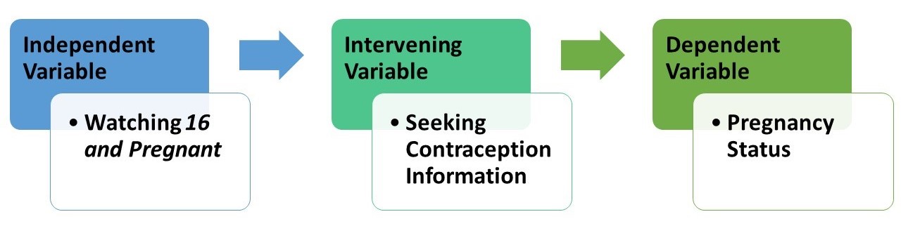
Before we go further we’d like to introduce you to three kinds of control variables: intervening, antecedent, and extraneous control variables. An intervening control variable is a variable a researcher believes is affected by an independent variable and in turn affects a dependent variable. The Latin root of “intervene” is intervener, meaning “to come between”—and that’s what intervening variables do. They come between, at least in the researcher’s mind, the independent and dependent variables.
For Kearney and Levine, seeking information about contraception was an intervening variable: it’s a variable they thought was affected by watching 16 and Pregnant (their independent variable) and in turn affected the likelihood that a young woman would be become pregnant (their dependent variable). More precisely, their three-variable hypothesis goes something like this: a young woman who watched 16 and Pregnant was more likely to seek information than a woman who did not watch it, and a woman who sought information about contraception was less likely to get pregnant than a woman who did not seek information about contraception. One quick way to map such a hypothesis is the following:
Importantly, researchers who believe they’ve found an intervening variable linking an independent variable and a dependent variable don’t believe they are challenging the possibility that the independent variable may be a cause of variation in the dependent variable. (More about “cause” in a second.) They are simply pointing to a possible way, or mechanism through which, the independent variable may cause or affect variation in the dependent variable.
A second kind of control variable is an antecedent variable. An antecedent variable is a variable that a researcher believes affects both the independent variable and the dependent variable. Antecedent has a Latin root that translates into “something that came before.” And that’s what researchers who think they’ve found an antecedent variable believe: that they’ve found a variable that not only comes before and affects both the independent variable and the dependent variable, but also, in some real sense, causes them to go together, or to be related.
Example
For an example of a researcher/theorist who thinks he may have found an antecedent variable that explains a relationship, think about what Robert Sternberg is saying about the correlation between the attractiveness of children and the care their parents give them in this article on the research by W. Andrew Harrell.
Quiz at the end of the article: What two variables constituted the independent and dependent variables of the finding announced by researchers at the University of Alberta? How did they show these two variables were related? What variable did Robert Sternberg suspect might have been an antecedent variable for the independent and dependent variables found to be related by the U. of Alberta researchers? How did he think this variable might explain the relationship?
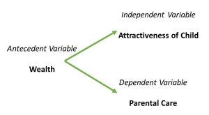
If you said that the basic relationship discovered by the University of Alberta researchers was that ugly children get poorer care from their parents than pretty children, you were right on the money. (It’s back-patting time!) Here the proposed independent variable was the attractiveness of children and the dependent variable was the parental care they received.
If you said that the socioeconomic status or wealth of the parents was what Sternberg thought might be an antecedent variable for these two variables (attractiveness and care), then you should glow with pride. Sternberg suggested that wealthier parents can both make their children look more attractive than poorer parents can and give their children better care than poorer parents can. One quick way to map such a hypothesis is like this:
A Word About Causation
Importantly, a researcher who thinks they have found an antecedent variable for a relationship implies that that have found a reason why the original relationship might be non-causal. Spurious is a word researchers use to describe non-causal relationships. Philosophers of science have told us that in order for a relationship between an independent variable and a dependent variable to be causal, three conditions must obtain:
1. The independent and dependent variables must be related. We demonstrated ways, using crosstabulation, that such relationships can be established with data. The Alberta researchers did show that the attractiveness of children was associated with how well they were treated (cared for or protected) in supermarkets. This condition is sometimes called association.
2. Instances of the independent variable occurring must come before, or at least not after, instances of the dependent variables. The attractiveness of the children in the Alberta study almost certainly preceded their treatment by their parents during the shopping expeditions observed by the researchers. This factor is often called temporal order.
3. There can be NO antecedent variable that creates the relationship between the independent variable and the dependent variable. This is the really tough condition for researchers to demonstrate, because, in principle, there could be an infinite numbers of antecedent variables that create such a relationship. This factor is often called elimination of alternatives. There is one research method—the controlled laboratory experiment—that theoretically eliminates this difficulty, but it is beyond the scope of this book to show you how. Yet it is not beyond our scope to show you how an antecedent variable might be shown, with data, to throw real doubt on the notion that an independent variable causes a dependent variable. And we’ll be doing that shortly.
Back to Our Main Story
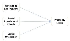
A third kind of control variable is an extraneous variable. An extraneous variable is a variable that has an effect on the dependent variable that is separate from the effect of the independent variable. One can easily imagine variables that would affect the chances of an adolescent woman’s getting pregnant (the dependent variable for Kearney and Levine) that have nothing to do with her having watched, or not watched, the TV show 16 and Pregnant. Whether or not friends are sexually active, and whether or not she defines herself as a lesbian, are two such variables. Sexual experience of her friendship group and sexual orientation, then, might be considered extraneous variables when considering the relationship between watching 16 and Pregnant and becoming pregnant. One might map the relationship among these four variables in the following way:
What Happens When You Control for a Variable and What Does it Mean?
You may be wondering how one could confirm any three-variable hypothesis with data. Let’s look at an example using data from eight imaginary adolescent women, whether they watched 16 and Pregnant, got pregnant, and sought information about contraception:
| Case | Watched Show | Got Pregnant | Sought Contraception Information |
| 1 | Yes | No | Yes |
| 2 | Yes | No | Yes |
| 3 | Yes | No | Yes |
| 4 | Yes | Yes | Yes |
| 5 | No | Yes | No |
| 6 | No | Yes | No |
| 7 | No | Yes | No |
| 8 | No | No | No |
Checking out a three-variable hypothesis requires, first, that you determine the relationship between the independent and dependent variables: in this case, between having watched 16 and Pregnant and pregnancy status. Do you recall how to do that? In any case, we’ve done it in Table 1.
Table 1. Crosstabulation of Watching 16 and Pregnant and Pregnancy Status
| Watched 16 and Pregnant | |||
| Yes | No | ||
| Got Pregnant | Yes | 1 (25%) | 3 (75%) |
| No | 3 (75%) | 1 (25%) | |
| |Yule’s Q|=0.80 | |||
You’ll note that the direction of this relationship, as expected by Kearny and Levine, is that women who had watched the show were less likely to get pregnant than those who had not. And a Yule’s Q of 0.80 suggests the relationship is strong.
What controlling a relationship for another variable means is that one looks at the original relationship (in this case between watching the show and becoming pregnant) after eliminating variation in the control variable. We eliminate such variation by separating out the cases that fall into each category of the control variable, and examining the relationship between the independent and dependent variables in each category. In this case, what this means is that we first look at the relationship between watching and getting pregnant for those who have sought contraceptive information and then look at it for those who have not sought such information. To do this we create two more tables that have the same form as Table 1, one into which only those who fell into the “yes” category of having sought contraceptive information are put, the other into which only those cases that fell into the “no” category of having sought contraceptive information are put. Doing this, we’ve created two more tables, Tables 2 and 3. Table 2 looks at the relationship between having watched the show and having become pregnant only for the four cases that sought contraceptive information; Table 3 does this only for the four cases that didn’t seek contraceptive information.
Table 2 Crosstabulation of Watching 16 and Pregnant and Pregnancy Status For Those Who Sought Contraceptive Information
| Watched 16 and Pregnant | |||
| Yes | No | ||
| Got Pregnant | Yes | 1 | 0 |
| No | 3 | 0 | |
| |Yule’s Q|=0.00 | |||
Table 3 Crosstabulation of Watching 16 and Pregnant and Pregnancy Status For Those Who Did Not Seek Contraceptive Information
| Watched 16 and Pregnant | |||
| Yes | No | ||
| Got Pregnant | Yes | 0 | 3 |
| No | 0 | 1 | |
| |Yule’s Q|=0.00 | |||
We call relationship between an independent and dependent variable for the part of a sample that falls into one category of a control variable a partial relationship or simply a partial. What is notable about the partial relationships in both Table 4.2 and 4.3 is that they are as weak as they could possibly be (both Yule’s Qs are equal to 0.00); both are much weaker than the original relationship between watching the show and becoming pregnant. In fact, in the context of controlling a relationship between two variables for a third, the relationship between the independent variable and the dependent variable, before the control, is often called an original relationship.
It may not surprise you to learn that controlling a relationship for a third variable does not always yield partials that are all weaker than the original. In fact, a famous methodologist, Paul Lazarsfeld (see Rosenberg, 1968), identified four distinct possibilities and others have called the resulting typology the elaboration model. Elaboration, in fact, is the term used by researchers for the process of controlling a relationship for a third variable. Table 4 outlines the basic characteristics of Lazarsfeld’s four types of elaboration, with one more thrown in because, as we’ll show, this fifth one is not only a logical, but also a practical, possibility.
Table 4. The Elaboration Model: Five Kinds of Elaboration
| Type of Elaboration | Kind of Control Variable | Relationship of Partials to the Original |
| Interpretation | Intervening | All partials weaker than the original |
| Replication | Doesn’t Matter | All partials about the same as the original |
| Explanation | Antecedent | All partials weaker than the original |
| Specification | Doesn’t Matter | Some, but not all, partials different (stronger and/or weaker) than the original |
| Revelation | Doesn’t Matter | All partials stronger than the original |
Quiz at the end of the table: What kind of elaboration is demonstrated, in your view, in Tables 4.1 to 4.3?
You may recall that Kearney and Levine saw seeking contraceptive information as an intervening variable between the watching of 16 and Pregnant and pregnancy status. Moreover, the partial relationships (shown in Tables 2 and 3) are both weaker than the original (shown in Table 1), so the elaboration shown in Tables 1 through 3 is an interpretation. If this kind of elaboration occurred in the real world, one could be pretty sure that seeking contraceptive information was indeed a mechanism through which watching the show affected a teenage woman’s pregnancy status. Note: while the quantitative result in cases of interpretation and explanation are the same, the explanations for the processes at work are different, and this means the researcher must rely on their own knowledge of the variables at hand to determine which is at work. In cases of interpretation, an intervening variable is at work, and thus the relationship between the independent and dependent variables is a real relationship—it’s just that the intervening variable is the mechanism through which this relationship occurs. In contrast, for cases of explanation, an antecedent variable is responsible for the apparent relationship between the independent and dependent variables, and thus this apparent relationship does not really exist. Rather, it is spurious.
In the real world, things don’t usually work out quite as neatly as they did in this example, where an original relationship completely “disappears” in the partials. If one finds evidence of an interpretation, it’s likely to be more subdued. Tables 5 and 6 demonstrate this point. Here, the researcher’s (Roger’s) hypothesis had been that people who are more satisfied with their finances are generally happier than people who are less satisfied. Table 5 uses General Social Survey (GSS) data to provide support for this hypothesis. Comparing percentages, about 47.5 percent of people who are satisfied with their finances claimed to be very happy, while only 17.3 percent who have claimed to be not at all satisfied with their finances said they were very happy. Moreover, a gamma of 0.42 suggests this relationship is in the hypothesized direction and that it is strong.
Table 5 Crosstabulation of Satisfaction with Finances and General Happiness, GSS Data from SDA
|
|||||||||||||||||||||||||||||||||||||||||||||||||||||||
|
|||||||||||||||||||||||||||||||||||||||||||||||||||||||
|
|||||||||||||||||||||||||||||||||||||||||||||||||||||||
Roger also introduced a control variable, the happiness of respondents’ marriages, believing that this variable might be an intervening variable for the relationship between financial satisfaction and general happiness. In fact, he hypothesized that people who are more satisfied with their finances would be happier in their marriages than people who were not satisfied with their finances, and that happily married people would be more generally happy than people who are not happy in their marriages. In terms of the elaboration model, he was expecting that the relationships between financial satisfaction and general happiness for each part of the sample defined by a level of marital happiness (i.e., the partials) would be weaker than the original relationship between financial satisfaction and general happiness. And (hallelujah!) he was right. Table 6 shows that the relationship between financial satisfaction and general happiness for those with very happy marriages yielded a gamma of 0.35; for those with pretty happy marriages, 0.33; and for those with not too happy marriages, 0.31. All three of the partial relationships were weaker than the original, which we showed in Table 5 had a gamma of 0.43.
Table 6. Gammas for the Relationship Between Satisfaction with Finances and General Happiness for People with Different Degrees of Marital Happiness
| Very Happy | Pretty Happy | Not Too Happy |
| 0.34 | 0.33 | 0.31 |
Because the partials for each level of marital happiness are only somewhat weaker than the original relationship between financial satisfaction and general happiness, they don’t suggest that marital satisfaction is the only reason for the relationship between financial satisfaction and general happiness, but they do suggest it is probably part of the reason. A curious researcher might look for others. But you get the idea: data can be used to shed light on the meaning of basic, two-variable relationships.
Perhaps more interesting still is that data can be used to resolve disputes about basic relationships. To illustrate, let’s return to the “Ugly Children” study and Alberta, discussed in the chapter on bivariate analysis. One of the Alberta researchers, a Dr. Harrell, essentially said the fact that prettier children got better care than uglier children was causal: parents with prettier children are propelled by evolutionary forces, in his view, to protect their children (and, one assumes, parents of uglier children are not). A Dr. Sternberg, however, didn’t see this relationship as causal. Instead, he saw it as the spurious result of wealth: wealthier parents can feed and clothe their kids better than others and are more likely to be caught up on supermarket etiquette associated with child care than others. Who’s right?
One way one could check this out is by collecting and analyzing data. Suppose, for instance, that a researcher replicated the Alberta study (following parent/child dyads around supermarkets to determine the attractiveness of the children and how well they were cared for), but added observations about the cars the parent/child couples came in. Late-model cars might be used as an indicator of relative wealth; beat-up dentmobiles (like Roger’s), of relative poverty. Then one could see how much of the relationship between attractiveness and care “disappeared” in the parts of the sample that were defined by wealth and poverty. Suppose, in fact, the data so collected looked like this:
Table 7. Hypothetical Data to Test Dr. Sternberg’s Hypothesis
| Case | Attractiveness | Care | Wealth |
| 1 | Pretty | Good | Rich |
| 2 | Pretty | Good | Rich |
| 3 | Pretty | Good | Rich |
| 4 | Pretty | Bad | Rich |
| 5 | Ugly | Bad | Poor |
| 6 | Ugly | Bad | Poor |
| 7 | Ugly | Bad | Poor |
| 8 | Ugly | Good | Poor |
Quiz about these data: Can you figure out the direction and strength of the relationship between the attractiveness of children and their care in this sample? What is the strength of this relationship within each category (rich and poor) of the control variable? What kind of elaboration did you uncover?
If you found that the original relationship was that pretty children got better care than ugly children (75% of the former did so, while only 25% of the latter did), you should be glowing with pride. If you found that the strength of the relationship (Yule’s Q=0.80) was strong, your brilliance is even more evident. And if you found that this strength “disappeared” (Yule’s Qs = 0.00) within each category of the wealth, you’re a borderline genius. If you decided that the elaboration is an “explanation,” because the partials are both weaker than the original and you’ve got an antecedent variable (at least according to Sternberg), you’ve crossed the border into genius.
Now referring back to the criteria for demonstrating causation (above), you’ll note that the third criterion was that there must not be any antecedent variable that creates the relationship between the independent and dependent variables. What this means in terms of data analysis is that there can’t be any antecedent variables whose control makes the relationship “disappear” within each of the parts of the sample defined by its categories. But that’s exactly what has happened above. In other words, one can show that a relationship is non-causal (or spurious) by showing, through data, that there is an antecedent variable whose control, as in the example we’ve just been working with, makes the relationship “disappear.” Pretty cool, huh?
On the other hand, while it’s impossible to use data to show that a relationship is causal,[1] it is possible to show that any single third variable that others hypothesize is creating the relationship between the relevant independent and dependent variables isn’t really creating that relationship. Thus, for example, Harrell and his Alberta team might have heard Sternberg’s claim that the wealth of “families” is the real reason why the attractiveness and care of children are related. And if they’d collected data like the following, they could have shown this claim was false. Can you use the data to do so? See if you can analyze the data and figure out what kind of elaboration Harrell et al. would have discovered.
Table 8. Hypothetical Data to Test Dr. Harrell
| Case | Attractiveness | Care | Wealth |
| 1 | Pretty | Good | Rich |
| 2 | Pretty | Good | Rich |
| 3 | Ugly | Good | Rich |
| 4 | Ugly | Bad | Rich |
| 5 | Pretty | Good | Poor |
| 6 | Pretty | Good | Poor |
| 7 | Ugly | Good | Poor |
| 8 | Ugly | Bad | Poor |
If you found that these data yielded a “replication,” you’re clearly on the brink of mastering the elaboration model. The original relationship between attractiveness and care was that pretty kids got better care than ugly kids (100% of pretty kids got it, compared to 50% of ugly kids who did) and this relationship was strong (Yule’s Q= 1.00). But each of the partials was just as strong (Yule’s Qs = 1.00), and had the same direction, as the original. What a replication shows is that the variable that was conceived of as an antecedent variable (wealth) does not “explain” the original relationship at all. The relationship is just as strong in each part of the sample defined by categories of the antecedent variable as it was before variation in this variable was controlled.
A Quick Word About Significance Levels
This chapter’s focus on the elaboration model and controlling relationships has been all about making comparisons: primarily about comparing the strength of partial relationships to the strength of original relationships (but sometimes, as you’ll soon see, comparing the strength of partials to one another). We haven’t said a thing about comparing inferential statistics and the resulting information about whether one dare generalize from a sample to the larger population from which the sample has been drawn. This has been intentional. You may recall (from the chapter on bivariate analyses) that the magnitude of chi-square is directly related to the size of the sample: the larger the sample, given the same relationship, the greater the chi-square. When one controls a relationship between an independent and dependent variable, however, one is dividing the sample into at least two parts, and, depending on the number of categories of the control variable, potentially more. So comparing the chi-squares, and therefore the significance levels, of partials to that of an original is hardly a fair fight. The originals will always involve more cases than the partials. So we usually limit our comparisons to those of strength (and sometimes direction), though if a relationship loses its statistical significance when examining the partials this does mean that the relationship cannot necessarily be generalized in its partial form.
Having made this important point, however, we’ll let you loose on the two quizzes that will end this chapter, each of which will introduce you to a new kind of elaboration.
Quiz #1 at the End of the Chapter
Show that the (hypothetical) sample data, below, conceivably collected to test Kearney and Levine’s three-variable hypothesis (that adolescents who watched the show were more likely to seek contraceptive information than others, and that those who sought information were less likely to get pregnant than others) are illustrative of a “specification.” For which category of the control variable (sought contraceptive information) is the relationship between having watched 16 and Pregnant and having gotten pregnant stronger? For which is it weaker? Why would such data NOT support Kearney and Levine’s hypothesis?[2]
| Case | Watched Show | Got Pregnant | Sought Contraceptive Information |
| 1 | Yes | No | Yes |
| 2 | Yes | No | Yes |
| 3 | No | Yes | Yes |
| 4 | No | Yes | Yes |
| 5 | Yes | Yes | No |
| 6 | Yes | No | No |
| 7 | No | Yes | No |
| 8 | No | No | No |
Quiz #2 at the End of the Chapter
| Case | Attractiveness | Care | Wealth |
| 1 | Pretty | Good | Rich |
| 2 | Pretty | Good | Rich |
| 3 | Ugly | Bad | Rich |
| 4 | Ugly | Bad | Rich |
| 5 | Pretty | Bad | Poor |
| 6 | Pretty | Bad | Poor |
| 7 | Ugly | Good | Poor |
| 8 | Ugly | Good | Poor |
Suppose the data you collected to test Sternberg’s hypothesis (that the relationship between the attractiveness of children and their care is a result of family wealth or social class) really looked like this ⇒
What kind of elaboration would you have uncovered? What makes you say so? (Doesn’t it seem odd that partial relationships can be stronger than original relationships? But they sure can. That what Roger calls a “revelation.”)
Exercises
- Write definitions, in your own words, for each of the following key concepts from this chapter:
-
multivariate analysis
-
antecedent variable
-
intervening variable
-
control variable
-
extraneous variable
-
spurious
-
original relationship
-
partial relationship
-
elaboration
-
interpretation
-
replication
-
explanation
-
specification
-
revelation
-
-
Below are real data from the GSS. See what you can make of them.
Who do you think would be more fearful of walking in their neighborhoods at night: males or females? Recalling that gamma= Yule’s Q for 2 x 2 tables, what does the following table, and its accompanying statistics, tell you about the actual direction and strength of the relationship? Support your answer with details from the table.
Table 9. Crosstabulation of Gender (Sex) with Whether Respondent Reports Being Fearful of Walking in the Neighborhood at Night (Fear), GSS Data from SDA
Frequency Distribution Cells contain:
–Column percent
-Weighted Nsex 1
male2
femaleROW
TOTALfear 1: yes 22.2
4,468.451.6
12,027.938.0
16,496.22: no 77.8
15,620.248.4
11,294.162.0
26,914.3COL TOTAL 100.0
20,088.6100.0
23,322.0100.0
43,410.6Means 1.78 1.48 1.62 Std Devs .42 .50 .49 Unweighted N 19,213 24,158 43,371 Color coding: <-2.0 <-1.0 <0.0 >0.0 >1.0 >2.0 Z N in each cell: Smaller than expected Larger than expected Summary Statistics Eta* = .30 Gamma = -.58 Rao-Scott-P: F(1,590) = 1,776.84 (p= 0.00) R = -.30 Tau-b = -.30 Rao-Scott-LR: F(1,590) = 1,828.11 (p= 0.00) Somers’ d* = -.29 Tau-c = -.29 Chisq-P(1) = 3,936.97 Chisq-LR(1) = 4,050.56 *Row variable treated as the dependent variable.
We controlled this relationship for “race,” a variable that had three categories: Whites, Blacks, and others. Suppose you learned that the gamma for this relationship among Whites was -0.61, among Blacks was -0.53 and among those identifying as members of other racial groups was -0.44. What kind of elaboration, in your view, would you have uncovered? Justify your answer.
- Please read the article by Robert Bartsch et al., entitled “Gender Representation in Television Commercials: Updating an Update” (Sex Roles, Vol. 43, Nos. 9/10, 2000: 735-743).[3] What is the main point of the article, in your view? What is the significance, according to Bartsch et al., of the gender of the voice-over in a commercial? Please examine Table 1 on page 739. Describe the overall gender breakdown of the voice-overs in 1998. Which gender was more represented in the voice-overs? Now look at the gender breakdown for voice-overs for domestic products and nondomestic products separately. Which of these is the stronger relationship: the one for domestic or the one for nondomestic products? What kind of elaboration would you say Bartsch et al. uncovered when they controlled the gender of voice-over for type of product (domestic or nondomestic)? How might you account for this finding?
Media Attributions
- Figure 4.1
- Figure 4.2
- Diagramming an Extraneous Variable Relationship © Mikaila Mariel Lemonik Arthur
- The reason you can never show, through data analysis, that a two-variable relationship is causal is that for every two-variable relationship there are an infinite number of possible antecedent variables, and we just don’t live long enough to test all the possibilities. ↵
- The original relationship, in this case, would be strong |Yule’s Q|= 0.80. The partial relationship for those who had sought contraception, however, would be stronger (|Yule’s Q|= 1.00, while that for those who had not sought contraception would be very weak (|Yule’s Q|= 0.00). You can specify, therefore, that the original relationship is particularly strong for those who’d sought contraception and particularly weak for those who had not. Kearney and Levine’s hypothesis had anticipated an “interpretation,” but this data yield a specification. So the data would prove their hypothesis wrong. ↵
- If the link below doesn’t work, perhaps you can hunt down an electronic copy of the article through your college’s library service. ↵
Quantitative analyses that explores relationships involving more than two variables or examines the impact of other variables on a relationship between two variables.
A variable that is neither the independent variable nor the dependent variable in a relationship, but which may impact that relationship.
A variable hypothesized to intervene in the relationship between an independent and a dependent variable; in other words, a variable that is affected by the independent variable and in turn affects the dependent variable.
A variable that is hypothesized to affect both the independent variable and the dependent variable.
The term used to refer to relationship where variables seem to vary in relation to one another, but where in fact no causal relationship exists.
The situation in which variables are able to be shown to be related to one another.
The order of events in time; in relation to causation, the fact that independent variables must occur prior to dependent variables.
In relation to causation, the requirement that for a causal relationship to exist, all possible explanations other than the hypothesized independent variable have been eliminated as the cause of the dependent variable.
A variable that impacts the dependent variable but is not related to the independent variable.
Examining a relationship between two variables while eliminating the effect of variation in an additional variable, the control variable.
A relationship between an independent and a dependent variable for only the portion of a sample that falls into a given category of a control variable.
Shorter term for a partial relationship.
The relationship between an independent variable and a dependent variable before controlling for an additional variable.
A typology developed by Paul Lazarsfeld for the possible analytical outcomes of controlling for a variable.
A term used to refer to the process of controlling for a variable.
