Quantitative Data Analysis
3 Univariate Analysis
Roger Clark
Univariate Analyses in Context
This chapter will introduce you to some of the ways researchers use statistics to organize their presentation of individual variables. In Exercise 1 of Introducing Social Data Analysis, you looked at one variable from the General Social Survey (GSS), “sex” or gender, and found that about 54 percent of respondents over the years have been female while about 46 percent have been male. You in fact did an analysis of one variable, sex or gender, and hence did an elementary univariate analysis.
Before we go further into your introduction to univariate analyses, we’d like to provide a somewhat larger context for it. In doing so, we begin with a number of distinctions. One distinction has to do with the number of variables that are involved in an individual analysis. In this book you’ll be exposed to three kinds of analysis: univariate, bivariate and multivariate analyses. Univariate analyses are ones that tell us something about one variable. You did one of these when you discovered that there have been more female than male respondents to the GSS over the years. Bivariate analyses, on the other hand, are analyses that focus on the relationship between two variables. We have just used the GSS source we guided you to (Thomas 2020/2021) to discover that over the years men have been much more likely to work full time than women—roughly 63 percent of male respondents have done so since 1972, while only about 40 percent of female respondents have. This finding results from a bivariate analysis of two variables: gender and work status. Multivariate analyses, then, are ones that permit the examination of the relationship between two variables while investigating the role of other variables as well. Thus, for instance, when we look at the relationship between gender and work status for White Americans and Black Americans separately, we are involving a third variable: race. For White Americans, the GSS tells us, about 63 percent of males have held full time jobs over time, while only about 39 percent of females have done so. For Black Americans, the difference is smaller: 56 percent of males have worked full time, while 44 percent of females have done so. We thus did a multivariate analysis, in which we examined the relationship between gender and work status, while also examining the effect of race on that relationship.
Another important distinction is between descriptive and inferential statistics. This distinction calls into play another: that between samples and populations. Many times researchers will use data that have been collected from a sample of subjects from a larger population. A population is a group of cases about which researchers want to learn something. These cases don’t have to be people; they could be organizations, localities, fire or police departments, or countries. But in case of the GSS, the population of interest is in fact people: all adults in the United States. Very often, it is impractical or undesirable for researchers to gather information about every subject in the population. You can imagine how much time and money it would cost for those who run the GSS, for instance, to contact every adult in the country. So what researchers settle for is information from samples of the larger population. A sample is a number of cases drawn from a larger population. In 2018, for instance, the organization that runs the GSS collected information on just over 2300 adult Americans.
Now we can address the distinction between descriptive and inferential statistics. Descriptive statistics are statistics used to describe a sample. When we learned, for instance, that the GSS reveals that about 63 percent of male respondents worked full time, while about 40 percent of female respondents worked full time, we were getting a description of the sample of adult Americans who had ever participated in the GSS. (And you’d be right if you added that this is a case of bivariate descriptive statistics, since the percentages describe the relationship between two variables in the sample—gender and work status. You’re so smart!) Inferential statistics, on the other hand, are statistics that permit researchers to make inferences about the larger populations from which the sample was drawn. Without going into too much detail here about the requirements for using inferential statistics[1] or how they are calculated, we can tell you that our analysis generated statistics that suggested we’d be on solid ground if we inferred from our sample data that a relationship between gender and work status not only exists in the sample, but also in the larger population of American adults from which the sample was drawn.
In this chapter we will learn something about both univariate descriptive statistics (statistics that describe single variables in a sample) and univariate inferential statistics (statistics that permit inferences about those variables in the larger population from which the sample was drawn).
Levels of Measurement of Variables
Now we can get down to basics. We’ve been throwing around the term variable as if it were second nature to you. (If it is, that’s great. If not, here we go.) A variable is a characteristic that can vary from one subject or case to another or for one case over time. In the case of the GSS data we’ve presented so far, one variable characteristic has been gender or sex. A human adult responding to the GSS may indicate that they are male or female. (They could also identify with other genders, of course, but the GSS hasn’t permitted this so far.) Gender is a variable because it is a characteristic that can vary from one human to another. If we were studying countries, one variable characteristic that might be of interest is the size of the population. Variables, we said, can also vary from one subject over time. Thus, for instance, your age is in one category today, but will be in another next year and in yet another in two years.
The nature of the kinds of categories is crucial to the understanding of the kinds of statistical analysis that can be applied to them. Statisticians refer to these “kinds” of categories as levels of measurement. There are four such levels or kinds of variables: nominal level variables, ordinal level variables, interval level variables, and ratio level variables. And, as you’ll see, the term “level” of measurement makes sense because each level requires that an additional criterion is met for distinguishing it from the previous “level.” The most basic level of measurement is that of the nominal level variable, or a variable whose categories have names. (The word “nominal” has the Latin root nomen, or name.) We say the nominal level is the most basic because every variable is at least a nominal variable. The variable “gender,” when it has the two categories, male and female, has categories that have names and is therefore nominal. So is “religion,” when it has categories like Protestant, Catholic, Jew, Muslim, and other. But so does the variable “age,” when it has categories from 1 and 2 to, potentially, infinity. Each one of categories (1,2,3, etc.) has a name, even though the name is a number. In other words, again, every variable is a nominal level variable. There are some nominal level variables that have the special property of only consisting of two categories, like yes and no or true and false. These variables are called binary variables (also known as dichotomous variables).
To be an ordinal level variable, a variable must have categories can be ordered in some sensible way. (The word “ordinal” has the Latin root ordinalis, or order.) Said another way, an ordinal level variable is a variable whose categories have names and whose categories can be ordered in some sensible way. An example would be the variable “height,” when the categories are “tall,” “medium,” and “short.” Clearly these categories have names (tall, medium and short), but they also can be ordered: tall implies more height than medium, which, in turn, implies more height than short. The variable “gender,” would not qualify as an ordinal level variable, unless one were an inveterate sexist, thinking that one gender is somehow a superior category to the others. Both nominal and ordinal level variables can be called discrete variables, which means they are variables measured using categories rather than numbers.
To be an interval level variable, a variable must be made up of adjacent categories that are a standard distance from one another, typically as measured numerically. Fahrenheit temperatures constitute an interval level variable because the difference between 78 and 79 degrees (1 degree) is seen as the same as the difference between 45 and 46 degrees. But because all those categories (78 degrees, etc.) are named and can be ordered sensibly, it’s pretty easy to see that all interval level variables could be measured at the ordinal level—even while not all nominal and ordinal level variables could be measured at the interval level.
Finally, we come to ratio level variables. Ratio variables are like interval level variables, but with the addition of an absolute zero, a category that indicates the absence of the phenomenon in question. And while some interval level variables cannot be multiplied and divided, ratio level variables can be. Age is an example of a ratio variable because the category, zero, indicates a person or thing has no age at all (while, in contrast, “year of birth” in the calendar system used in the United States does not have an absolute zero, because the year zero is not the absence of any years). But, while interval and ratio variables can be distinguished from each other, we are going to assert that, for the purposes of this book, they are so similar that the distinction isn’t worth insisting upon. As a result, for practical purposes, we could be calling all interval and ratio variables, interval-ratio variables, or simply interval variables. Both ratio and interval level variables can also be referred to as scale or continuous variables, as their (numerical) categories can be placed on a continuous scale.
But what are those practical purposes for which we need to know a variable’s level of measurement? Let’s just see . . .
Measures of Central Tendency
Roger likes to say, “All statistics are designed with particular levels of measurement in mind.” What’s this mean?[2] Perhaps the easiest way to illustrate is to refer to what statisticians call “measures of central tendency” or what we laypersons call “averages.” You may have already learned about three of these averages before: the mean, the median, and the mode. But have you asked yourself why we need three measures of central tendency or average?
The answer lies in the level of measure required by each kind of average. The mean (which is what people most typically refer to when they use the term “average”), you may recall, is the sum of all the categories (or values) in your sample divided by the number of such categories (or values). Now, stop and think: what level of measurement (nominal, ordinal or interval) is required for you to calculate a mean?
If your answer was “interval,” you should give yourself a pat on the back.[3] You need a variable whose categories may legitimately be added to one another in order to calculate a mean. You could do this with the variable “age,” whose categories were 0, 1, 2, 3, etc. But you couldn’t, say, with “height,” if the only categories available to you were tall, medium, and short (if you had actual height in inches or centimeters, of course, that would be a different story).
But if your variable of interest were like that height variable—i.e., an ordinal level variable, statisticians have cooked up another “average” or measure of central tendency just for you: the median. The median is the middle category (or value) when all categories (or values) in the sample are arranged in order. Let’s say your five subjects had heights that were classified as tall, short, tall, medium and tall. If you wanted to calculate the median, you’d first arrange these in order as, for instance, short, medium, tall, tall and tall. You’d then pick the one in the middle—i.e., tall—and that would be your median. Now, stop and think: could you calculate the median of an interval level variable, like the age variable we just talked about?
If your answer was “yes,” you should give yourself a hardy slap on the knee.[4] The median can be used to analyze an interval level variable, as well as ordinal level variables, because all interval level variables are also ordinal. Right?
OK, you say, the mean has been designed to summarize interval level variables and the median has been fashioned to handle ordinal level variables. “I’ll bet,” you say, “the mode is for analyzing nominal level variables.” And you’re right! The mode is the category of a variable in a sample that occurs most frequently. This can be calculated for nominal level variables because nominal level variables, whatever else they have, have categories (with names). Let’s say the four cars you were studying had the colors of blue, red, green and blue. The mode would be blue, because it’s the category of colors that occurs most frequently. Before you take these averages out for a spin, we’d like you to try another question. Can a mode be calculated on an ordinal or an interval level variable?
If you answer “yes,” you should be very proud. Because you’ve probably seen that ordinal and interval variables could also be treated like nominal level variables and therefore can have modes. (That is, categories that occur most frequently). Note, though, that the mode is unlikely to be a helpful measure in instances where continuous variables have many possible numerical values, like annual income in dollars, because in these cases the mode might just be some dollar amount made by three people in a sample where everyone else’s income is unique.
Your Test Drive
| Student | A | B | C | D | E |
| Religion | Catholic | Protestant | Jewish | Catholic | Catholic |
| Height | Tall | Short | Medium | Short | Short |
| Age | 19 | 20 | 19 | 21 | 19 |
How do you know which measure of central tendency or average (mode, median or mean) to use to describe a given variable in a report? The first rule is a negative: do NOT report a measure that is not suitable for your variable’s level of measurement. Thus, you shouldn’t report a mean for the religion or height variables in the “test drive” above, because neither of them is an interval level variable.
You might well ask, “How could I possibly report a mean religion, given the data above?” This is a good question and leads us to mention, in passing, that when researchers set up computer files to help them analyze data, they will almost always code variable categories using numbers so that the computer can recognize them more easily. Coding is the process of assigning observations to categories—and, for computer usage, this often means changing the names of variables categories to numbers. Perhaps you recall doing Exercise 1 at the end of Introducing Social Data Analysis—the one that asked you to determine the percentage of respondents who were female over the years (about 54 percent). Well, to set up the computer to do this analysis, the folks who created the file (and who supplied us with the data) coded males as 1 and females as 2. So the computer was faced with over 34,000 1s and 2s rather than with over 34,000 “males” and “females.” Computers like this kind of help. But computers, while very good at computing, are often a little stupid when it comes to interpreting their computations.[6] So when I went in and asked the computer to add just a few more statistics, including the mean, median and mode, about the sex or gender of GSS respondents, it produced this table. (Don’t worry, I’ll show you how to produce a table like this in Exercise 3 of this chapter.)
| Summary Statistics | |||||||
|
Mean = |
1.54 |
|
Std Dev = |
.50 |
|
Coef var = |
.32 |
|
Median = |
2.00 |
|
Variance = |
.25 |
|
Min = |
1.00 |
|
Mode = |
2.00 |
|
Skewness = |
-.17 |
|
Max = |
2.00 |
|
Sum = |
99,993.48 |
|
Kurtosis = |
-1.97 |
|
Range = |
1.00 |
What this table effectively and quickly, tells us is that the mode of “sex” (really gender) is 2, meaning “female.” Part of your job as a social data analyst is to translate codes like this back into English—and report that the mode, here, is “female,” not “2”. But another important part, and something the computer also cannot do, is recognizing the level of measure of the variable concerned—in this case, nominal—and realize which of the reported statistics is relevant given that level. And in terms of “sex,” as reported in Table 1, only you can know how silly it would be to report that the mean “sex” is 1.54 (notice the computer can’t see that silliness) or that its median is 2.00. When Roger was little,[7] Smoky the Bear used to tell kids “Only YOU can prevent forest fires.” But Roger is here to tell you, “Only YOU can prevent statistical reporting travesties.” So, again, you do not want to report statistics that aren’t designed for the level of measure of your variables.
In general, though, when you ARE dealing with an interval variable, like age in years, you really have three choices about which to report: the mean, the median and the mode. For the moment, we’re going to recommend that, in such case, you might consider that the reading public is likely to be most familiar with the mean and, for that reason, you might report the mean. (We’ll get to qualifications of that recommendation a little later.)
Variation
Measures of central tendency are often useful for summarizing variables, but they can sometimes be misleading. Roger just[8] Googled the average life expectancy for men in the United States and discovered it was about 76.5 years. (Pretty clearly a mean, not a mode or median, right?) At this sitting, he is about 71.5 years old. Does this mean he has exactly 5 years left of life to live? Well, probably not. Given his health, educational level, etc., he’s likely to live considerably longer…unless COVID-19 gets him tomorrow. The point is that for life expectancy, as for other variables, there’s variation around the average. And sometimes knowing something about that variation is at least as important as the average itself—sometimes more important.
We can learn a lot about a variable, for instance, simply by showing how its cases are distributed over its categories in a sample. Exercise 1 at the end of Introducing Social Data Analysis actually told you the modal gender of respondents to the GSS survey. (“Modal” is the adjectival form of mode.) Do you recall what that was? It was “female,” right? What this tells you is that the “average” respondent over the years has been a female. But the mode, being what it is, doesn’t tell you whether 100 percent of respondents were female or 50.1 percent were female. And that’s an important difference.
One of the most commonly used ways of showing variation is what’s called a frequency distribution. A frequency distribution shows the number of times cases fall into each category in a sample. I’ve just called up the table you looked at in Exercise 1 of Introducing Social Data Analysis and plunked it down here as Table 2. What this table shows is that while about 35,179 females had participated in the GSS since 1972, 29,635 males had done so as well. The table further tells us that while about 54 percent of the sample is female, about 46 percent has been male. The distribution has been much closer to 50-50 than 100-0. And this extra information about the variable is a significant addition to the fact that modal “sex” was female.
| Frequency Distribution | ||
| Cells contain: –Column percent -Weighted N |
Distribution | |
| SEX |
1: MALE |
45.7 |
|
2: FEMALE |
54.3 |
|
|
COL TOTAL |
100.0 |
|
“Sex” is a nominal level variable, and frequency distributions have been designed for displaying the variation of nominal level variables. But, of course, because ordinal and interval variables are also nominal level variables, frequency distributions can be used to describe their variation as well. And this often makes sense with ordinal level variables. Thus, for instance, we used a frequency distribution of respondents’ confidence in the military (“conarm”) to show that there was relatively little variation in Americans’ confidence in that institution in 2018 (Table 3, below). Almost 61 percent of respondents said they had a “great deal of confidence” in the military that year, while only about 39 percent said they had “only some” or “hardly any” confidence. In other words, at least in comparison with the variation in “sex,” variation in confidence in the military, which, after all, has three categories, seems limited. In other words, this kind of confidence seems more concentrated in one category (“great deal of confidence”) than you might expect.
Quiz at the End of the Paragraph: Can you see what the median and the mode of confidence in the military was?
Bonus Trick Question: What was its mean?
| Frequency Distribution | ||
| Cells contain: –Column percent -Weighted N |
Distribution | |
|
CONARMY (Confidence in the U.S. Military) |
1: A GREAT DEAL |
60.6 |
|
2: ONLY SOME |
32.5 |
|
|
3: HARDLY ANY |
7.0 |
|
|
COL TOTAL |
100.0 |
|
| Summary Statistics | ||||||
|
Mean = |
1.46 |
Std Dev = |
.62 |
|
Coef var = |
.43 |
|
Median = |
1.00 |
Variance = |
.39 |
|
Min = |
1.00 |
|
Mode = |
1.00 |
Skewness = |
1.00 |
Max = |
3.00 |
|
|
Sum = |
2,273.32 |
Kurtosis = |
-.06 |
|
Range = |
2.00 |
Measures of Variation for Interval Level Variables
Looking at frequency distributions is a pretty good way of getting a sense of the variation in nominal and ordinal variables. But it would be a fairly awkward way of doing so for interval variables, many of which, if you think about it, would have many categories. (Can you imagine a frequency distribution for the variable “age” of respondents in the GSS?) Statisticians have actually given us some pretty elegant ways of dealing with the description of variation in interval variables and we’d now like to illustrate them with simple examples.
Roger’s daughter, Wendy, was a day care provider for several years and could report that variation in the ages of preschool children made a tremendous difference in the kinds of things you can do with them. Imagine, if you will, that you had two groups of four preschool children, one of which had four 3-year-olds in it and one of which had two 5-year-olds and two 1-year-olds. Can you calculate the mean age of each group?
If you found that the mean age of both groups was 3 years old, you did a fine job. Now, if you were inclined to think that any two groups with the same mean age were likely to be similar, think of these two from a day care provider’s point of view. Figuring out what to do for a day with two 1-year-olds and two 5-year-olds would be a much more daunting task than planning for four 3-year-olds. Wouldn’t it?
Statisticians have given us one particularly simple measure of spread or variation for interval level variables: the range. The range is simply the highest category in your sample minus the lowest category. For the group with four 3-year-olds, the range would be (3-3=) zero years. There is no variation in age for this group. For the group with two 1-year-olds and two 5-year-olds, the range would be (5-1=) four years. A substantial, and important difference, again especially if you, like my daughter, were a day care provider. Means don’t always tell the whole story, do they?
Perhaps the more commonly used statistic for describing the variation or spread of an interval level variable, however, is the standard deviation. The range only gives you a sense of how spread out the extreme values or categories are in your sample. The standard deviation is a measure of variation that takes into account every value’s distance from the sample mean. The usefulness of such a measure can be illustrated with another simple example. Imagine, for instance, that your two groups of preschool children had the following ages: 1, 1, 5, 5, on the one hand, and 1, 3, 3, and 5, on the other.
The mean of these two groups is 3 years and the range is 4 years. But are they identical? No. You may notice that each of the individual ages in the first group is a “distance” of 2 away from the mean of 3. (The two 1s are each 2 away from 3 and the two 5s are also 2 away from 3.) So the average “distance” of each age from the mean is 2 for group 1. But that’s not true for the second group. The 1 and the 5 are both 2 away from the mean of 3, but the two 3s are both no distance away. So the average distance of ages from the mean in this group is something less than 2. Hence, the average distance of ages from the mean in the first group is larger than the average distance in the second group. The standard deviation is a way of capturing a difference like this—one that is not captured by the range.
It does this by using a formula that essentially adds the individual “distances” of categories or values from the mean and then divides that number by the categories. We think of it as being very similar to the computation of the mean itself: a sum divided by the number of cases involved. The computational formula is:
[latex]SD_{sample} = \sqrt{\frac{ \sum_{i=1}^N (x - \overline{x})^2} {N-1} }[/latex]
where [latex]SD_{sample}[/latex] stands for the standard deviation
[latex]\sqrt{~^{~}}[/latex] stands for the square root of the entire expression that follows
[latex]\sum_{i=1}^N[/latex] means to add up the sequence of numbers produced by the expression that follows
[latex]x[/latex] stands for each value of category in the sample
[latex]\overline{x}[/latex] stands for the sample mean
[latex]N[/latex] stands for the number of sample cases
The formula may look daunting, but it’s not very difficult to compute with just a few cases—and we’ll never ask you to use anything other than a computer to compute the standard deviation with more cases. Note that to calculate the standard deviation for an entire population, rather than a sample, we use N rather than N-1 in the denominator. And also note that the numerator—[latex]Var(X)=\sum_{i=1}^N (x - \overline{x})^2[/latex]—is referred to as the variance.
Notice first that the formula asks you to compute the sample mean. For the second sample of ages above—the one with ages 1, 3, 3, 5—the mean is 3. It then asks you to take the difference between each category in the sample and the mean and square the differences. 1-3, for instance, is -2 and its square is 4. 3-3 is 0 and its square is 0. And 5-3 is 2 and its square is 4. The formula then asks you to add these squared values up: 4 0 0 4=8. Then it says to divide by the number of cases, minus 1: 3. 8/3=2.67. It then asks you to take the square root of 2, or about 1.6. So the standard deviation of this sample is about 1.6 years.
Can you calculate the standard deviation for the second sample of ages above: 1, 1, 5, 5?
Did you get 2.3? If so, give yourself another pat on the back.[9]
Measures of Deviation from the Normal Distribution
We’ve suggested that, other things being equal, the mean is a good way of describing the central tendency or average of an interval level variable. But other things aren’t always equal. The mean is an excellent measure of central tendency, for instance, when the interval level variable conforms to what is called a normal distribution. A normal distribution of a variable is one that is symmetrical and bell-shaped (otherwise called a bell curve), like the one in Figure 2.1. This image suggests what is true when the distribution of a variable is normally distributed: that 68 percent of cases fall within one standard deviation on either side of the mean; that 95 percent of the cases fall within two standard deviations on either side; and that 99.7 percent of the cases fall within three standard deviations on either side. Note that the symbol [latex]\sigma[/latex] is used to indicate standard deviation in many statistical contexts.
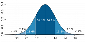
One example that is frequently cited as a normally distributed variable is height. For American men, the average height in 2020 is about 69 inches,[10] where “average” here refers to the mean, the median and the mode, if, in fact, height is normally distributed. The peak of the curve (can you see it in your mind?) would be at 69 inches, which would be the most frequently occurring category, the one in the middle of the distribution of categories and the arithmetic mean.
But what happens when a variable is not normally distributed? We asked the Social Data Archive to use GSS data from 2010 to tell us what distribution of the number of children respondents had looked like, and we got these results (see Table 4):
| Summary Statistics | |||||||
|
Mean = |
1.91 |
|
Std Dev = |
1.73 |
Coef var = |
.91 |
|
|
Median = |
2.00 |
|
Variance = |
2.99 |
Min = |
.00 |
|
|
Mode = |
.00 |
|
Skewness = |
1.05 |
Max = |
8.00 |
|
|
Sum = |
3,894.30 |
|
Kurtosis = |
1.39 |
Range = |
8.00 |
|
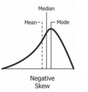
As you might have expected, the greatest number of respondents said they had zero, one or two children. But, then the number of children tails off pretty quickly as you get into categories that represent respondents with 3 or more children. This variable, then, is not normally distributed. Most of the cases are concentrated in the lowest categories. When an interval level variable looks that this, it is said to have right, or positive skewness, and this is reflected in the report that “number of children” has a skewness of positive 1.05. Skewness refers to an asymmetry in a distribution in which a curve is distorted either to the left or the right. The skewness statistic can take on values from negative infinity to positive infinity, with positive values indicating right skewness (with “tails” to the right) and negative values indicating left skewness (when “tails” are to the left). A skewness statistic of zero would indicate that a variable is perfectly symmetrical.
Our rule of thumb is that when the skewness statistic gets near to 1 or near -1, the variable has more than enough skewness (either to the right or to the left) to be disqualified as a normally distributed variable. And in such cases, it’s probably useful to report both the mean and the median as measures of central tendency, since the relationship of the two will give some idea to readers of the nature of the variable’s skewness. If the median is greater than the mean (as it is in the case of “number of children”), it’s a sign that the author means to convey that the variable is right skewed. If it’s less than the mean, the implication is that it’s left skewed.
Kurtosis refers to how sharp the peak of a frequency distribution is. If the peak is too pointed to be a normal curve, it is said to have positive kurtosis (or “leptokurtosis”). The kurtosis statistic of “number of children” is 1.39, indicating that the variable’s distribution has positive kurtosis (or leptokurtosis). If the peak of a distribution is too flat to be normally distributed, it is said to have negative kurtosis (or platykurtosis), as seen in Figure 2.3.
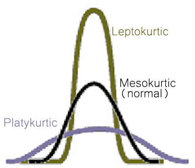
A rule of thumb for the kurtosis statistic: if it gets near to 1 or near -1, the variable has more than enough kurtosis (either positive or negative) to be disqualified as a normally distributed variable.
For a fascinating, personal lecture about the importance of being wary about reports using only measures of central tendency or average (e.g., means and medians), however, we encourage you to listen to the following talk by Stephen Jay Gould:
A Word About Univariate Inferential Statistics
Up to this point, we’ve only talked about univariate descriptive statistics, or statistics that describe one variable in a sample. When we learned that 54 percent of GSS respondents over the years have been women, we were simply learning about the (large) sample of people who have responded to the GSS over the years. And when we learned that the mean number of children that respondents had in 2010 was about 1.9 and the median was 2.0, those too were descriptions of the sample that year. One of the purposes of sampling, though, is that it can provide us some insight into the population from which the sample was drawn. In order to make inferences about such populations from sample data we need to use inferential statistics. Inferential statistics, as we said before, are statistics that permit researchers to make inferences about the larger population from which a sample is drawn.
We’ll be spending more time on inferential statistics in other chapters, but now we’d like to introduce you a statistical concept that frequently comes up in relation to political polls: margin of error. To appreciate the concept of the margin of error, we need to understand the difference between two important concepts: statistics and parameters. A statistic is a description of a variable (or the relationship between variables) in a sample. The mean, median, mode, range, standard deviation and skewness are all types of statistics. A parameter, on the other hand, is a description of a variable (or the relationship between variables) in a population; many (but not all) of the same tools used as statistics when analyzing data from samples can be used as parameters when analyzing data on populations. A margin of error, then, is a suggestion of how far away from the actual population parameter a statistic is likely to be. Thus political polling can tell you precisely what percentage of the sample say they are going to vote for a candidate, but it can’t tell you precisely what percentage would say the same thing in the larger population from which the sample was drawn.
BUT, when a sample is a probability sample of the larger population, we can estimate how close the population percentage is likely to be to the sample percentage. A full discussion of the different kinds of samples is beyond the scope of this book, but let’s just say that a probability sample is one that has been drawn to give every member of the population a known (non-zero) chance of inclusion. Inferential statistics of all kinds assume that one is dealing with a probability sample of the larger population to which one would like to generalize (though, sometimes, inferential statistics are calculated even when this fundamental assumption of inferential statistics has not been met).[11]
Most frequently, a margin of error is a statement of the range around the sample percentage in which there is a 95 percent chance that the population percentage will fall. The pre-election polls before the 2016 election are frequently criticized for how badly they got it wrong when they predicted Hillary Clinton would get a higher percentage of the vote than Donald Trump—and win the election. But in fact most of the national polls came remarkably close to predicting the election outcome perfectly. Thus, for instance, an ABC News/Washington Post poll, collected between November 3rd and November 6th (two days before the election), and involving a sample of 2,220, predicted that Clinton would get 49 percent of the vote, plus or minus 2.5 percentage points (meaning that she’d likely get somewhere between 46.5 percent and 51.5 percent of the vote), and that Trump would get 46 percent, plus or minus 2.5 percentage points (meaning that he’d likely get somewhere between 43.5 percent and 48.5 percent of the vote). The margin of error in this poll, then, was plus or minus 2.5 percentage points. And, in fact, Clinton won 48.5 percent of the actual vote (well within the margin of error) and Trump won 46.4 percent (again, well within the margin of error) (CNN Politics, 2020). This is just one poll that got the election precisely right with respect to the total vote (if not the crucial electoral vote) count in advance of the election.
We haven’t shown you how to calculate a margin of error here but, as you’ll see in Exercise 4 at the end of the chapter, they are not hard to get a computer to spit out. One thing to keep in mind is that the size of a margin of error is a function of the size of the sample: the larger the sample, the smaller the margin of error. In fact all inferences using inferential statistics become more accurate as the sample size increases.
So, welcome to the world of univariate statistics! Now let’s try some exercises to see how they work.
Exercises
-
- Which of the measures of central tendency has been designed for nominal level variables? For ordinal level variables? For interval level variables? Why can all three measures be applied to interval level variables?
- Which way of showing the variation of nominal and ordinal level variables have we examined in this chapter? What measures of variation for interval level variables have we encountered?
- Return to the Social Data Archive we explored in Exercise 1 of Introducing Social Data Analysis. The data, again, are available at https://sda.berkeley.edu/ . Again, go down to the second full paragraph and click on the “SDA Archive” link you’ll find there. Then scroll down to the section labeled “General Social Surveys” and click on the first link there: General Social Survey (GSS) Cumulative Datafile 1972-2018 release. Now type “religion” in the row box, hit “output options,” click on “summary statistics,” then click on “run the table.” See if you can answer these questions:
-
-
- What level of measurement best characterizes “religion”? What is this variable measuring?
- What’s the only measure of central tendency you can report for “religion”? Report this measure, in English, not as a number.
- What’s a good way you can describe ”religion”’s variation? Describe its variation.
-
Now type “happy” in the row box, hit “output options,” click on “summary statistics,” then click on “run the table.” See if you can answer these questions:
-
-
- What level of measurement best characterizes “happy”? What is this variable measuring?
- What are the only measures of central tendency you can report for “happy”? Report these measures, in English, not as a number.
- What’s a good way you can use to describe “happy”’s variation? Describe its variation.
-
Now type “age” in the row box, hit “output options,” click on “summary statistics,” then click on “run the table.” See if you can answer these questions:
-
-
- What level of measure best describes “age”? What is this variable measuring?
- What are all the measures of central tendency you could report for “age”? Report these measures, in English, not simply as numbers.
- What are two good statistics for describing “age”’s variation? Describe its variation.
- Is it your sense that “age” is essentially normally distributed? Why or why not? (What statistics did you check for this?)
-
- Return to the Social Data Archive. The data, again, are available at https://sda.berkeley.edu/ (You may have to copy and paste this address to request the website.) Again, go down to the second full paragraph and click on the “SDA Archive” link you’ll find there. Then scroll down to the section labeled “American National Election Studies (ANES)” and hit on the first link there: American National Election Study (ANES) 2016. These data come from a survey done after the 2016 election. Type “Trumpvote” in the row, hit “output options,” and hit “confidence intervals,” then hit “run table.” What percentage of respondents, after the election, said they had voted for Trump? What was the “95 percent” confidence interval for this percentage? Check the end of this chapter for the actual percentage of the vote that Trump got. Does it fall within this interval?
Media Attributions
- Standard_deviation_diagram.svg © M. W. Toews is licensed under a CC BY (Attribution) license
- Negative Skew © Diva Dugar adapted by Roger Clark is licensed under a CC BY-SA (Attribution ShareAlike) license
- Kurtosis © Mikaila Mariel Lemonik Arthur
- Note that you can use many statistical methods to analyze data about populations, there are some differences in how they are employed, as will be discussed later in this chapter. ↵
- Besides the fact that he’s getting increasingly senile? ↵
- Something that’s increasingly difficult for Roger to do as he gets up in years. ↵
- Unless you’ve got arthritis there like you know who. ↵
- The mode of religion is Catholic. No other average is applicable. The median of height is short, and so is the mode. The mean of height can’t be calculated. The mean height is 19.6. Its median is 19, as is its mode. ↵
- No offense to you, my faithful laptop, without which I couldn’t bring you, my readers, this cautionary tale. ↵
- Many years ago. ↵
- In 2020. ↵
- You already know Roger can’t do this for himself. ↵
- 5 feet, 9 inches ↵
- And we hope you’ll always say “naughty, naughty,” when you know this has been done. ↵
Quantitative analyses that tell us about one variable, like the mean, median, or mode.
Quantitative analyses that tell us about the relationship between two variables.
Quantitative analyses that explores relationships involving more than two variables or examines the impact of other variables on a relationship between two variables.
Statistics used to describe a sample.
Statistics that permit researchers to make inferences (or reasoned conclusions) about the larger populations from which a sample has been drawn.
A subset of cases drawn or selected from a larger population.
A group of cases about which researchers want to learn something; generally, members of a population share common characteristics that are relevant to the research, such as living in a certain area, sharing a certain demographic characteristic, or having had a common experience.
A characteristic that can vary from one subject or case to another or for one case over time within a particular research study.
Classification of variables in terms of the precision or sensitivity in how they are recorded.
A variable whose categories have names that do not imply any order.
Consisting of only two options. Also known as dichotomous.
Consisting of only two options. Also known as binary.
A variable with categories that can be ordered in a sensible way.
A variable measured using categories rather than numbers, including binary/dichotomous, nominal, and ordinal variables.
A variable with adjacent, ordered categories that are a standard distance from one another, typically as measured numerically.
A numerical variable with an absolute zero which can also be multiplied and divided.
A variable measured using numbers, not categories, including both interval and ratio variables. Also called a continuous variable.
A variable measured using numbers, not categories, including both interval and ratio variables. Also called a scale variable.
A measure of the value most representative of an entire distribution of data.
The sum of all the values in a list divided by the number of such values.
The middle value when all values in a list are arranged in order.
The category in a list that occurs most frequently.
The process of assigning observations to categories.
An analysis that shows the number of cases that fall into each category of a variable.
The highest category in a list minus the lowest category.
A measure of variation that takes into account every value’s distance from the sample mean.
A distribution of values that is symmetrical and bell-shaped.
A graph showing a normal distribution—one that is symmetrical with a rounded top that then falls away towards the extremes in the shape of a bell
An asymmetry in a distribution in which a curve is distorted either to the left or the right, with positive values indicating right skewness and negative values indicating left skewness.
How sharp the peak of a frequency distribution is. If the peak is too pointed to be a normal curve, it is said to have positive kurtosis (or “leptokurtosis”). If the peak of a distribution is too flat to be normally distributed, it is said to have negative kurtosis (or platykurtosis).
The characteristic of a distribution that is too pointed to be a normal curve, indicated by a positive kurtosis statistic.
The characteristic of a distribution that is too flat to be a normal curve, indicated by a negative kurtosis statistic.
Quantitative measures of data from a sample.
A quantitative measure of data from a population.
A suggestion of how far away from the actual population parameter a sample statistic is likely to be.
A sample that has been drawn to give every member of the population a known (non-zero) chance of inclusion.
