Quantitative Data Analysis With SPSS
14 Quantitative Analysis with SPSS: Multivariate Crosstabs
Mikaila Mariel Lemonik Arthur
Producing a multivariate crosstabulation is exactly the same as producing a bivariate crosstabulation, except that an additional variable is added. Note that, due to the limitations of the crosstabulation approach, you are not actually looking at the relationships between all three variables simultaneously (and this approach is limited to three variables). Rather, you are looking at how controlling for a third variable—your “Layer” or control variable—changes the relationship between the independent and dependent variable in your analysis. What SPSS produces, then, is basically a stack of crosstabulation tables with your independent and dependent variables, one for each category of your control variable, along with statistical significance and association values for each category of your control variable. This chapter will review how to produce and interpret a multivariate crosstabulation. It uses variables with fairly few categories for ease of interpretation. Do note that when using variables with many categories, results can become quite complex and lengthy, and due to small numbers of cases left in each cell of the very lengthy tables, statistical significance is likely to be reduced. Thus, analysts should take care to consider whether the relationship(s) they are interested in are suitable for this type of analysis, and may want to consider recoding variables (see the chapter on data management) with many categories into somewhat fewer categories to facilitate analysis.
To produce a multivariate crosstabulation, follow the same steps as you
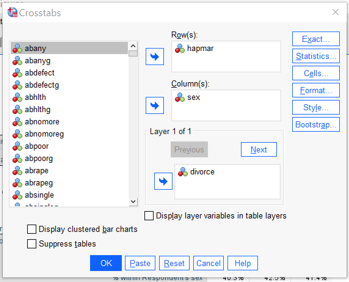
would follow to produce a bivariate crosstabulation—put the independent variable in the columns box, the dependent variable in the rows box, select column percentages under cells, and select chi square and an appropriate measure of association under statistics. Note that the measure of association you choose should be the same one that you would choose for a bivariate analysis with the same independent and dependent variables, as the third variable is a control variable and does not alter the criteria upon which the decision about measures of association is made. The one thing you need to add in order to produce a multivariate crosstabulation is that you add your third variable, the control variable, to the Layer box in the crosstabs dialog. Figure 1 shows what this would look like for a crosstabulation with the independent variable SEX, the dependent variable HAPMAR, and the control variable DIVORCE. In other words, this analysis is exploring whether being male or female influences respondents’ feelings of happiness in their marriages, controlling for whether or not they have ever been divorced.
| Ever been divorced or separated | Respondent’s sex | Total | ||||
|---|---|---|---|---|---|---|
| male | female | |||||
| yes | Happiness of R’s marriage | very happy | Count | 136 | 133 | 269 |
| % within Respondent’s sex | 57.1% | 52.8% | 54.9% | |||
| pretty happy | Count | 96 | 107 | 203 | ||
| % within Respondent’s sex | 40.3% | 42.5% | 41.4% | |||
| not too happy | Count | 6 | 12 | 18 | ||
| % within Respondent’s sex | 2.5% | 4.8% | 3.7% | |||
| Total | Count | 238 | 252 | 490 | ||
| % within Respondent’s sex | 100.0% | 100.0% | 100.0% | |||
| no | Happiness of R’s marriage | very happy | Count | 467 | 439 | 906 |
| % within Respondent’s sex | 65.6% | 59.8% | 62.7% | |||
| pretty happy | Count | 224 | 260 | 484 | ||
| % within Respondent’s sex | 31.5% | 35.4% | 33.5% | |||
| not too happy | Count | 21 | 35 | 56 | ||
| % within Respondent’s sex | 2.9% | 4.8% | 3.9% | |||
| Total | Count | 712 | 734 | 1446 | ||
| % within Respondent’s sex | 100.0% | 100.0% | 100.0% | |||
| Total | Happiness of R’s marriage | very happy | Count | 603 | 572 | 1175 |
| % within Respondent’s sex | 63.5% | 58.0% | 60.7% | |||
| pretty happy | Count | 320 | 367 | 687 | ||
| % within Respondent’s sex | 33.7% | 37.2% | 35.5% | |||
| not too happy | Count | 27 | 47 | 74 | ||
| % within Respondent’s sex | 2.8% | 4.8% | 3.8% | |||
| Total | Count | 950 | 986 | 1936 | ||
| % within Respondent’s sex | 100.0% | 100.0% | 100.0% | |||
| Ever been divorced or separated | Value | df | Asymptotic Significance (2-sided) | |
|---|---|---|---|---|
| yes | Pearson Chi-Square | 2.231b | 2 | .328 |
| Likelihood Ratio | 2.269 | 2 | .322 | |
| Linear-by-Linear Association | 1.649 | 1 | .199 | |
| N of Valid Cases | 490 | |||
| no | Pearson Chi-Square | 6.710c | 2 | .035 |
| Likelihood Ratio | 6.748 | 2 | .034 | |
| Linear-by-Linear Association | 6.524 | 1 | .011 | |
| N of Valid Cases | 1446 | |||
| Total | Pearson Chi-Square | 8.772a | 2 | .012 |
| Likelihood Ratio | 8.840 | 2 | .012 | |
| Linear-by-Linear Association | 8.200 | 1 | .004 | |
| N of Valid Cases | 1936 | |||
| a. 0 cells (0.0%) have expected count less than 5. The minimum expected count is 36.31. | ||||
| b. 0 cells (0.0%) have expected count less than 5. The minimum expected count is 8.74. | ||||
| c. 0 cells (0.0%) have expected count less than 5. The minimum expected count is 27.57. | ||||
| Ever been divorced or separated | Value | Approximate Significance | ||
|---|---|---|---|---|
| yes | Nominal by Nominal | Phi | .067 | .328 |
| Cramer’s V | .067 | .328 | ||
| N of Valid Cases | 490 | |||
| no | Nominal by Nominal | Phi | .068 | .035 |
| Cramer’s V | .068 | .035 | ||
| N of Valid Cases | 1446 | |||
| Total | Nominal by Nominal | Phi | .067 | .012 |
| Cramer’s V | .067 | .012 | ||
| N of Valid Cases | 1936 | |||
First, consider the crosstabulation table. As you can see, this table really consists of three tables stacked on top of each other. Each of these three tables considers the relationship between sex and the happiness of the respondent’s marriage, but there is one table for those who have ever been divorced, one table for those who have never been divorced, and one table for everyone. Comparing the percentages across the rows, we can make the following observations:
- Among those who have ever been divorced, males are slightly more likely to be very happy in their marriage, while females are somewhat more likely to be not too happy.
- Among those who have not ever been divorced, males are more likely to be very happy in their marriage, while females are more likely to be pretty happy and are somewhat more likely to be not too happy.
- Among the entire sample, males are more likely to be very happy in their marriages, while females are more likely to be pretty happy and somewhat more likely to be not too happy.
- Overall, then, the results suggest men are happier in their marriages than women.
Next, we turn to statistical significance. At the p<0.05 level, we can observe that this analysis produces significant results for those who have never been divorced and for the entire sample, but not for those who have been divorced. Turning to the association, we find a weak association—the figures for those who have been divorced, those who have not been divorced, and the entire population are quite similar.
Thus, we can conclude that women who have never been divorced are, on average, less happy in their marriages than men who have never been divorced, but that among those who have been divorced, the relationship between sex and marital happiness is not statistically significant.
Exercises
Select three variables of interest. Answer the following questions:
- Which is the independent variable, which is the dependent variable, and which is the control variable?
- What is the research hypothesis for this analysis? What do you predict will be the relationship between the independent variable and the dependent variable, and how will the control variable impact this relationship?
- What is the null hypothesis for this analysis?
- What confidence level (p value) have you chosen?
- Which measure of association is most appropriate for this relationship?
Next, use SPSS to produce a multivariate crosstabulation according to the instructions in this chapter. Interpret the crosstabulation. First, answer the following questions for each of the stacked crosstabulations of your independent and dependent variable (one for each category of the control variable, plus one for everyone):
- Is the relationship between the independent and dependent variables statistically significant?
- Can the null hypothesis be rejected?
- How strong is the association between the two variables?
- Looking at that pattern of percentages across the rows, what can you determine about the nature of the relationship between the two variables?
Then, compare your results across the different categories of the control variable.
- What does this tell you about how the control variable impacts the relationship between the independent and dependent variables?
- Is there support for your research hypothesis?
Media Attributions
- crosstabs dialog multivariate © IBM SPSS is licensed under a All Rights Reserved license
