Quantitative Data Analysis With SPSS
18 Quantitative Analysis with SPSS: Multivariate Regression
Mikaila Mariel Lemonik Arthur
In the chapter on Bivariate Regression, we explored how to produce a regression with one independent variable and one dependent variable, both of which are continuous. In this chapter, we will expand our understanding of regression. The regressions we produce here will still be linear regressions with one continuous dependent variable, but now we will be able to include more than one independent variable. In addition, we will learn how to include discrete independent variables in our analysis.
In fact, producing and interpreting multivariate linear regressions is not very different from producing and interpreting bivariate linear regressions. The main differences are:
- We add one or more additional variables to the Block 1 of 1 box (where the independent variables go) when setting up the regression analysis,
- We check off one additional option under Statistics when setting up the regression analysis, Collinearity diagnostics, which will be explained below,
- We interpret the strength and significance of the entire regression and then look at the strength, significance, and direction of each included independent variable one at a time, so there are more things to interpret, and
- We can add or remove variables and compare the R2 to see how those changes impacted the overall predictive power of the regression.
Each of these differences between bivariate and multivariate regression will be discussed below, beginning with the issue of collinearity and the tools used to diagnose it.
Collinearity
Collinearity refers to the situation in which two independent variables in a regression analysis are closely correlated with one another (when more than two independent variables are closely correlated, we call it multicollinearity). This is a problem because when the correlation between independent variables is high, the impact of each individual variable on the dependent variable can no longer be separately calculated. Collinearity can occur in a variety of circumstances: when two variables are measuring the same thing but using different scales; when they are measuring the same concept but doing so slightly differently; or when one of the variables has a very strong effect on the other.
Let’s consider examples of each of these circumstances in turn. If a researcher included both year of birth and age, or weight in pounds and weight in kilograms, both of the variables in each pair are measuring the exact same thing. Only the scales are different. If a researcher included both hourly pay and weekly pay, or the length of commute in both distance and time, the correlation would not be quite as close. A person might get paid $10 an hour but work a hundred hours per week, or get paid $100 an hour but work ten hours per week, and thus still have the same weekly pay. Someone might walk two miles to work and spend the same time commuting as someone else driving 35 miles on the highway. But overall, the relationships between hourly pay and weekly pay and the relationship between commute distance and commute time are likely to be quite strong. Finally, consider a researcher who includes variables measuring the grade students earned on Exam 1 and their total grade in a course with three exams, or one who includes variables measuring families’ spending on housing each month and their overall spending each month. In these cases, the variables are not measuring the same underlying phenomena, but the first variable likely has a strong effect on the second variable, resulting in a strong correlation.
In many cases, the potential for collinearity will be obvious when considering the variables included in the analysis, as in the examples above. But it is not always obvious. Therefore, researchers need to test for collinearity when performing multivariate regressions. There are several ways to do this. First of all, before beginning to run a regression, researchers can check for collinearity by running a correlation matrix and a scatterplot matrix to look at the correlations between each pair of variables. The instructions for these techniques can be found in the chapter on Quantitative Analysis with SPSS: Correlation. A general rule of thumb is that if a Pearson correlation is above 0.8, this suggests a likely problem with collinearity, though some suggest scrutinizing those pairs of variables with a correlation above 0.7.
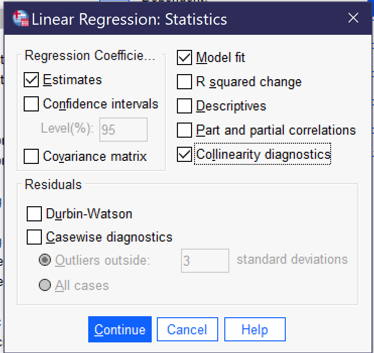
In addition, when running the regression, researchers can check off the option for Collinearity diagnostics (Alt+l) under the statistics dialog (Alt+S), as shown in Figure 1. The resulting regression’s Coefficients table will include two additional pieces of information, the VIF and the Tolerance, as well as an additional table called Collinearity diagnostics. The VIF, or Variance Inflation Factor, calculates the degree of collinearity present. Values of around or close to one suggest no collinearity; values around four or five suggest that a deeper look at the variables is needed, and values at ten or above definitely suggest collinearity great enough to be problematic for the regression analysis. The Tolerance measure calculates the extent to which other independent variables can predict the values of the variable under consideration; for tolerance, the smaller the number, the more likely that collinearity is a problem. Typically, researchers performing relatively straightforward regressions such as those detailed in this chapter do not need to rely on the Collinearity diagnostics table, as they will be able to determine which variables may be correlated with one another by simply considering the variables and looking at the Tolerance and VIF statistics.
Producing & Interpreting Multivariate Linear Regressions
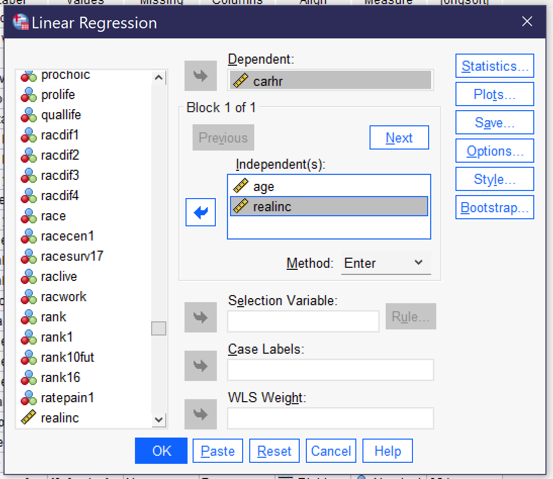
Producing multivariate linear regressions in SPSS works just the same as producing bivariate linear regressions, except that we add one or more additional variables to the Block 1 of 1 box and check off the Collinearity diagnostics, as shown in Figure 2. Let’s continue our analysis of the variable CARHR, adding the independent variable REALINC (inflation-adjusted family income) to the independent variable AGE. Figure 2 shows how the linear regression dialog would look when set up to run this regression, with CARHR in the Dependent box and AGE and REALINC in the Independent(s) box under Block 1 of 1. Be sure that Estimates, Model fit, and Collinearity diagnostics are checked off, as shown in Figure 1. Then click OK to run the regression.
Tables 1, 2, and 3 below show the results (excluding those parts of the output unnecessary for interpretation.
| Model | R | R Square | Adjusted R Square | Std. Error of the Estimate |
|---|---|---|---|---|
| 1 | .124a | .015 | .014 | 8.619 |
| a. Predictors: (Constant), R’s family income in 1986 dollars, Age of respondent | ||||
| Model | Sum of Squares | df | Mean Square | F | Sig. | |
|---|---|---|---|---|---|---|
| 1 | Regression | 1798.581 | 2 | 899.290 | 12.106 | <.001b |
| Residual | 114913.923 | 1547 | 74.282 | |||
| Total | 116712.504 | 1549 | ||||
| a. Dependent Variable: How many hours in a typical week does r spend in a car or other motor vehicle, not counting public transit | ||||||
| b. Predictors: (Constant), R’s family income in 1986 dollars, Age of respondent | ||||||
| Model | Unstandardized Coefficients | Standardized Coefficients | t | Sig. | Collinearity Statistics | |||
|---|---|---|---|---|---|---|---|---|
| B | Std. Error | Beta | Tolerance | VIF | ||||
| 1 | (Constant) | 9.808 | .752 | 13.049 | <.001 | |||
| Age of respondent | -.055 | .013 | -.106 | -4.212 | <.001 | 1.000 | 1.000 | |
| R’s family income in 1986 dollars | -1.356E-5 | .000 | -.064 | -2.538 | .011 | 1.000 | 1.000 | |
| a. Dependent Variable: How many hours in a typical week does r spend in a car or other motor vehicle, not counting public transit | ||||||||
So, how do we interpret the results of our multivariate linear regression? First, look at the Collinearity Statistics in the Coefficients table (here, Table 3). As noted above, to know we are not facing a situation involving collinearity, we are looking for a VIF that’s lower than 5 and a Tolerance that is close to 1. Both of these conditions are met here, so collinearity is unlikely to be a problem. If it were, we would want to figure out which variables were overly correlated and remove at least one of them. Next, we look at the overall significance of the regression in the ANOVA table (here, Table 3). The significance shown is <0.001, so the regression is significant. If it were not, we would stop there.
To find out the overall strength of the regression, we look at the R in the Model Summary (here, Table 1). It is 0.124, which means it is moderately strong. The R2 is 0.015, which—converting the decimal into a percentage by multiplying it by 100—tells us that the two independent variables combined explain 1.5% of the variance in the dependent variable, how much time the respondent spends in the car. And here’s something fancy you can do with that R2: compare it to the R2 for our prior analysis in the chapter on Bivariate Regression, which had just the one independent variable of AGE. That R2 was 0.10, so though our new regression still explains very little of the variance in hours spent in the car, adding income does enable us to explain a bit more of the variance. Note that you can only compare R2 values among a series of models with the same dependent variable. If you change dependent variables, you can no longer make that comparison.
Now, let’s turn back to the Coefficients table. When we interpreted the bivariate regression results, we saw that the significance and Beta values in this table were the same as the significance value in the ANOVA table and the R values, respectively. In the multivariate regression, this is no longer true—because now we have multiple independent variables, each with their own significance and Beta values. These results allow us to look at each independent variable, while holding constant (controlling for) the effects of the other independent variable(s). Age, here, is significant at the p<0.001 level, and its Beta value is -0.106, showing a moderate negative association. Family income is significant at the p<0.05 level, and its Beta value is -0.064, showing a weak negative association. We can compare the Beta values to determine that age has a larger effect (0.106 is a bigger number than 0.064; we ignore sign when comparing strength) than does income.
Next, we look at the B values to see the actual numerical effect of each variable. For every year of additional age, respondents spend on average 0.055 fewer hours in the car, or about 1.65 minutes less. And for every dollar of additional family income, respondents spend -1.356E-5 fewer hours in the car. But wait, what does -1.356E-5 mean? It’s a way of writing numbers that have a lot of decimal places so that they take up less space. Written the long way, this number is -0.00001356—so what the E-5 is telling us is to move the decimal point five spaces over. That’s a pretty tiny number, but that’s because an increase of $1 in your annual family income really doesn’t have much impact on, well, really anything. If instead we considered the impact of an increase of $10,000 in your annual family income, we would multiply our B value by $10,000, getting -0.1356. In other words, an increase of $10,000 in annual family income (in constant 1986 dollars) is associated with an average decrease of 0.1356 hours in the car, or a little more than 8 minutes.
Our final step is to create the regression equation. We do this the same way we did for bivariate regression, only this time, there is more than one x, so we have to indicate the coefficient and significance of each one separately. Some people do this by numbering their xs with subscript numerals (e.g. x1, x2, and so on), while others just use the short variable name. We will do the later here. Taking the numbers from the B column, our regression equation is
[latex]y=9.808-0.055AGE^{***}-1.356E-5REALINCOME^{*}[/latex].
Phew, that was a lot to go through! But it told us a lot about what is going on with our dependent variable, CARHR. That’s the power of regression: it tells us not just about the strength, significance, and direction of the relationship between a given pair of variables, but also about the way adding or removing additional variables changes things as well as about the actual impact each independent variable has on the dependent variable.
Dummy Variables
So far, we have reviewed a number of the advantages of regression analysis, including the ability to look at the significance, strength, and direction of the relationships between a series of independent variables and a dependent variable; examining the effect of each independent variable while controlling for the others; and seeing the actual numerical effect of each independent variable. Another advantage is that it is possible to include independent variables that are discrete in our analysis. However, they can only be included in a very specific way: if we transform them into a special kind of variable called a dummy variable in which a single value of interest is coded as 1 and all other values are coded as 0. It is even possible to create multiple dummy variables for different categories of the same discreet variable, so long as you have an excluded category or set of categories that are sizable. It is important to leave a sizeable group of respondents or datapoints in the excluded category because of collinearity.
Consider, for instance, the variable WRKSLF, which asks if respondents are self-employed or work for someone else. This is a binary variable, with only two answer choices. We could make a dummy variable for self-employment, with being self-employed coded as 1 and everything else (which, here, is just working for someone else) as 0. Or we could make a dummy variable for working for someone else, with working for someone else coded as 1 and everything else as 0. But we cannot include both variables in our analysis because they are, fundamentally, measuring the same thing.
Figuring out how many dummy variables to make and which ones they should be can be difficult. The first question is theoretical: what are you actually interested in? Only include categories you think would be meaningfully related to the outcome (dependent variable) you are considering. Second, look at the descriptive statistics for your variable to be sure you have an excluded category or categories. If all of the categories of the variable are sufficiently large, it may be enough to exclude one category. However, if a category represents very few data points—say, just 5 or 10 percent of respondents—it may not be big enough to avoid collinearity. Therefore, some analysts suggest using one of the largest categories, assuming this makes sense theoretically, as the excluded category.
Let’s consider a few examples:
| GSS Variable | Answer Choices & Frequencies | Suggested Dummy Variable(s) |
| RACE | White: 78.2% Black: 11.6% Other: 10.2% |
Option 1. 2 variables: Back 1, all others 0 & Other 1, all others 0 |
| Option 2. Nonwhite 1, all others 0 | ||
| Option 3. White 1, all others 0 | ||
| DEGREE | Less than high school: 6.1% High school: 38.8% Associate/junior college: 9.2% Bachelor’s: 25.7% Graduate: 18.8% |
Option 1. Bachelor’s or higher 1; all others 0 |
| Option 2. High school or higher 1; all others 0 | ||
| Option 3. 4 variables: Less than high school 1, all others 0; Associate/junior college 1, all others 0; Bachelor’s 1, all others 0; Graduate 1, all others 0 | ||
| Option 4. Use EDUC instead, as it is continuous | ||
| CHILDS | 0: 29.2% 1: 16.2% 2: 28.9% 3: 14.5% 4: 7% 5: 2% 6: 1.3% 7: 0.4% 8 or more: 0.5% |
Option 1. 0 children 1, all others 0 |
| Option 2. 2 variables: 0 children 1, all others 0; 1 child 1, all others 0 | ||
| Option 3. 3 variables: 0 children 1, all others 0; 1 child 1, all others 0; 2 children 1, all others 0 | ||
| Option 4. Ignore the fact that this variable is not truly continuous and treat is as continuous anyway | ||
| CLASS | Lower class: 8.7% Working class: 27.4% Middle class: 49.8% Upper class: 4.2% |
The best option is to create thee variables: Lower class 1, all others 0; Working class 1, all others 0; Upper class 1, all others 0 (however, you could instead include Working class and have a variable for Middle class if that made more sense theoretically) |
| SEX | Male: 44.1% Female: 55.9% |
Option 1. Male 1, all others 0 |
| Option 2: Female 1, all others 0 |
So, how do we go about making our dummy variable or variables? We use the Recode technique, as illustrated in the chapter on Quantitative Analysis with SPSS: Data Management. Just remember to Recode into different and to make as many dummy variables as needed: maybe one, maybe more. Here, we will make one for SEX. Because we are continuing our analysis of CARHRS, let’s assume we hypothesize that, on average, women spend more time in the car than men because women are more likely to be responsible for driving children to school and activities. On the basis of this hypothesis, we would treat female as the included category (coded 1) and male as the excluded category (coded 0) since what we are interested in is the effect of being female.
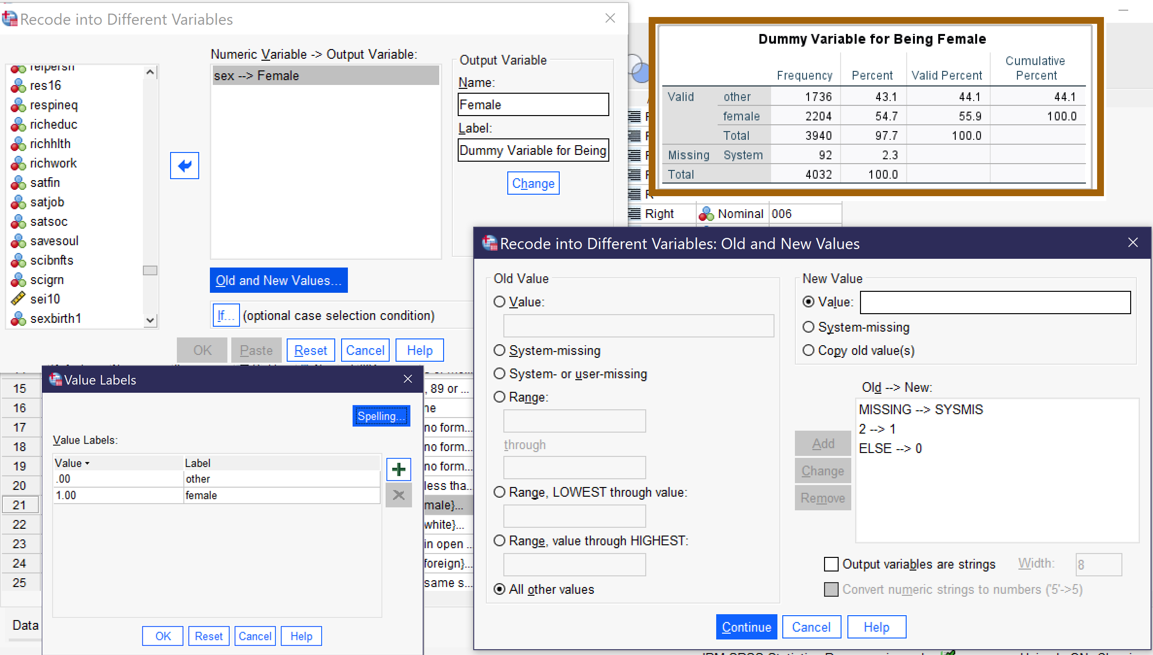
As a reminder, to recode, we first make sure we know the value labels for our existing original variable, which we can find out by checking Values in Variable View. Here, male is 1 and female is 2. Then we go to Transform → Recode into Different Variables (Alt+T, Alt+R). We add the original variable to the box, and then give our new variable a name, here generally something like the name of the category we are interested in (here, Female) and descriptive label, and click Change. Next, we click “Old and New Values.” We set system or user missing as system missing, our category of interest as 1, and everything else as 0. We click continue, then go to the bottom of variable view and edit our value labels to reflect our new categories. Finally, we run a frequency table of our new variable to be sure everything worked right. Figure 3 shows all of the steps described here.
Dummy Variables in Regression Analysis
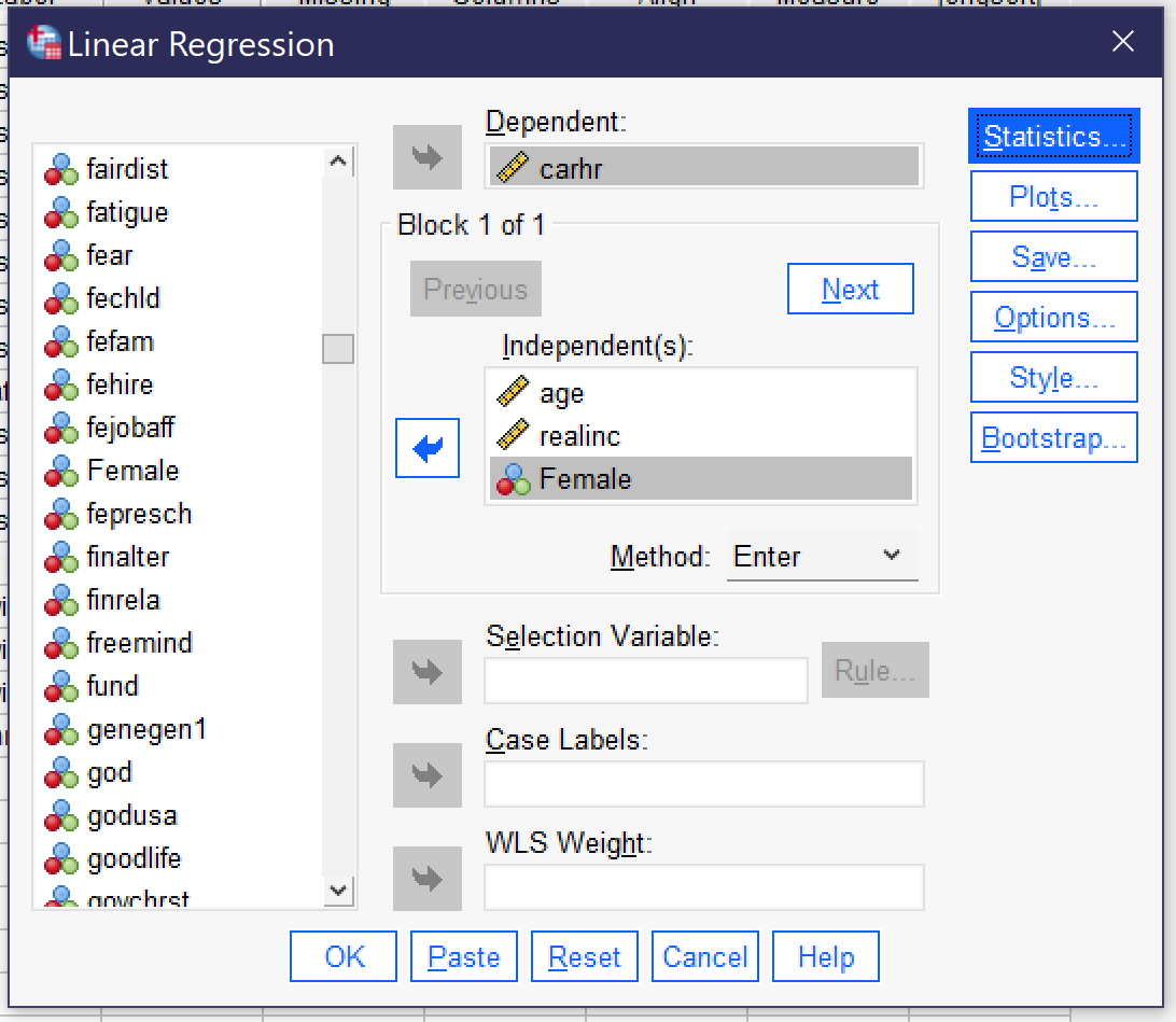
After creating the dummy variable, we are ready to include our dummy variable in a regression. We set up the regression just the same way as we did above, except that we add FEMALE to the independent variables REALINC and AGE (the dependent variable will stay CARHR). Be sure to check Collinearity diagnostics under Statistics. Figure 4 shows how the linear regression dialog should look with this regression set up. Once the regression is set up, click ok to run it.
Now, let’s consider the output, again focusing only on those portions of the output necessary to our interpretation, as shown in Tables 5, 6, and 7.
| Model | R | R Square | Adjusted R Square | Std. Error of the Estimate |
|---|---|---|---|---|
| 1 | .143a | .020 | .018 | 8.602 |
| a. Predictors: (Constant), Dummy Variable for Being Female, Age of respondent, R’s family income in 1986 dollars | ||||
| Model | Sum of Squares | df | Mean Square | F | Sig. | |
|---|---|---|---|---|---|---|
| 1 | Regression | 2372.292 | 3 | 790.764 | 10.686 | <.001b |
| Residual | 114259.126 | 1544 | 74.002 | |||
| Total | 116631.418 | 1547 | ||||
| a. Dependent Variable: How many hours in a typical week does r spend in a car or other motor vehicle, not counting public transit | ||||||
| b. Predictors: (Constant), Dummy Variable for Being Female, Age of respondent, R’s family income in 1986 dollars | ||||||
| Model | Unstandardized Coefficients | Standardized Coefficients | t | Sig. | Collinearity Statistics | |||
|---|---|---|---|---|---|---|---|---|
| B | Std. Error | Beta | Tolerance | VIF | ||||
| 1 | (Constant) | 10.601 | .801 | 13.236 | <.001 | |||
| Age of respondent | -.056 | .013 | -.108 | -4.301 | <.001 | 1.000 | 1.000 | |
| R’s family income in 1986 dollars | -1.548E-5 | .000 | -.073 | -2.882 | .004 | .986 | 1.014 | |
| Dummy Variable for Being Female | -1.196 | .442 | -.069 | -2.706 | .007 | .986 | 1.015 | |
| a. Dependent Variable: How many hours in a typical week does r spend in a car or other motor vehicle, not counting public transit | ||||||||
First, we look at our collinearity diagnostics in the Coefficients table (here, Table 7). We can see that all three of our variables have both VIF and Tolerance close to 1 (see above for a more detailed explanation of how to interpret these statistics), so it is unlikely that there is a collinearity problem.
Second, we look at the significance for the overall regression in the ANOVA table (here, Table 6). We find the significance is <0.001, so our regression is significant and we can continue our analysis.
Third, we look at the Model Fit table (here, table 5). We see that the R is 0.143, so the regression’s strength is moderate, and the R2 is 0.02, meaning that all of our variables together explain 2% of the variance (0.02 * 100 converts the decimal to a percent) in our dependent variable. We can compare this 2% R2 to the 1.5% R2 we obtained from the earlier regression without Female and determine that adding the dummy variable for being female helped our regression explain a little bit more of the variance in time respondents spend in the car.
Fourth, we look at the significance and Beta values in the Coefficients table. First, we find that Age is significant at the p<0.001 level and that it has a moderate negative relationship with time spent in the car. Second, we find that income is significant at the p<0.01 level and has a weak negative relationship with time spent in the car. Finally, we find that being female is significant at the p<0.01 level and has a weak negative relationship with time spent in the car. But wait, what does this mean? Well, female here is coded as 1 and male as 0. So what this means is that when you move from 0 to 1—in other words from male to female—the time spent in the car goes down (but weakly). This is the opposite of what we hypothesized! Of the three variables, age has the strongest effect (the largest Beta value).
Next, we look at the B values to see what the actual numerical effect is. For every one additional year of age, time spent in the car goes down by 0.056 hours (3.36 minutes) a week. For every one additional dollar of income, time spent in the car goes down by -1.548E-5 hours per week; translated (as we did above), this means that for every $10,000 additional dollars of income, time spent in the car goes down by 0.15 hours (about 9 minutes) per week. And women, it seems, spend on average 1.196 hours (about one hour and twelve minutes) fewer per week in the car than do men.
Finally, we produce our regression equation. Taking the numbers from the B column, our regression equation is [latex]y=10.601-0.056AGE^{***}-1.584E-5REALINCOME^{**}-1.196FEMALE^{**}[/latex].
Regression Modeling
There is one more thing you should know about basic multivariate linear regression. Many analysts who perform this type of technique systematically add or remove variables or groups of variables in a series of regression models (SPSS calls them “Blocks”) to look at how they influence the overall regression. This is basically the same as what we have done above by adding a variable and comparing the R2 (the difference between the two R2 values is called the R2 change). However, SPSS provides a tool for running multiple blocks at once and looking at the results. When looking at the Linear regression dialog, you may have noticed that it says “Block 1 of 1” just above the box where the independent variables go. Well, if you click “next” (Alt+N), you will be moved to a blank box called “Block 2 of 2”. You can then add additional independent variables here as an additional block.
Just below the Block box is a tool called “Method” (Alt+M). While a description of the options here is beyond the scope of this text, this tool provides different ways for variables in each block to be entered or removed from the regression to develop the regression model that is most optimal for predicting the dependent variable, retaining only those variables that truly add to the predictive power of the ultimate regression equation. Here, we will stick with the “Enter” Method, which does not draw on this type of modeling but instead simply allows us to compare two (or more) regressions upon adding an additional block (or blocks) of variables.
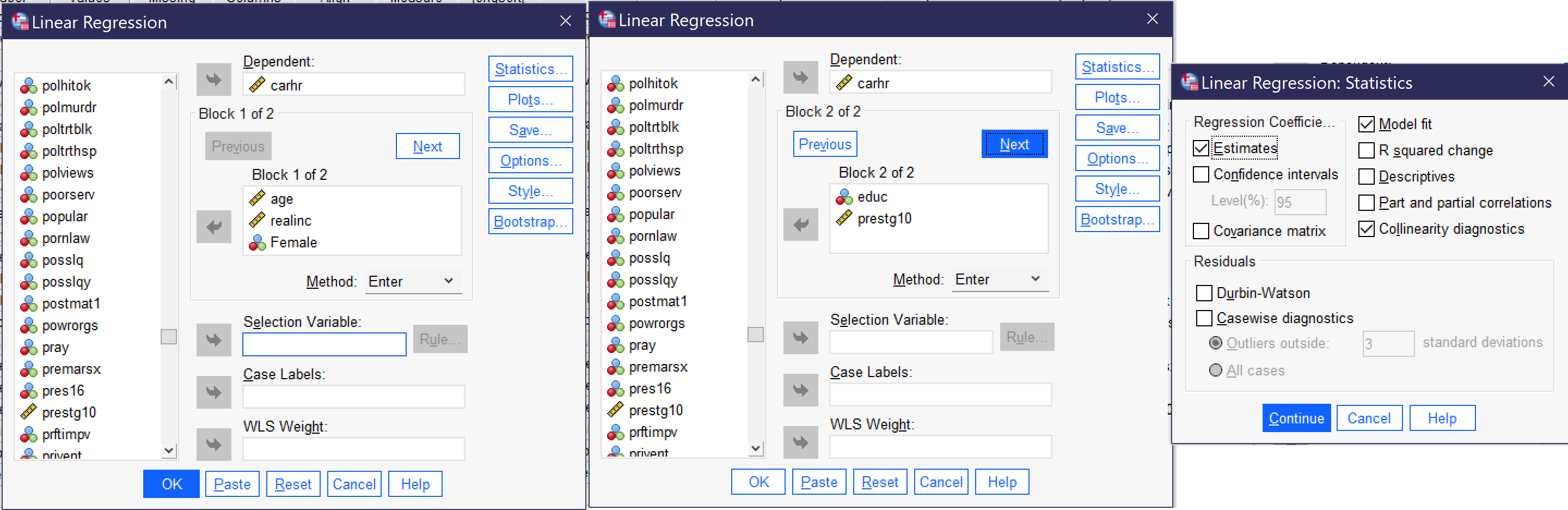
So, to illustrate this approach to regression analysis, we will retain the same set of variables for Block 1 that we used above: age, income, and the dummy variable for being female. And then we will add a Block 2 with EDUC (the highest year of schooling completed) and PRESTIG10 (the respondent’s occupational prestige score)[1]. Remember to be sure to check the collinearity diagnostics box under statistics. Figure 5 shows how the regression dialog should be set up to run this analysis.
The output for this type of analysis (relevant sections of the output appear as Tables 8, 9, and 10) does look more complex at first, as each table now has two tables stacked on top of one another. Note the output will first, before the relevant tables, include “Variables Entered/Removed” table that simply lists which variables are included in each block. This is more important for the more complex methods other than Enter in which SPSS calculates the final model; here, we already know which variables we have included in each block.
| Model | R | R Square | Adjusted R Square | Std. Error of the Estimate |
|---|---|---|---|---|
| 1 | .155a | .024 | .022 | 8.201 |
| 2 | .200b | .040 | .037 | 8.139 |
| a. Predictors: (Constant), Dummy Variable for Being Female, Age of respondent, R’s family income in 1986 dollars | ||||
| b. Predictors: (Constant), Dummy Variable for Being Female, Age of respondent, R’s family income in 1986 dollars, R’s occupational prestige score (2010), Highest year of school R completed | ||||
| Model | Sum of Squares | df | Mean Square | F | Sig. | |
|---|---|---|---|---|---|---|
| 1 | Regression | 2486.883 | 3 | 828.961 | 12.326 | <.001b |
| Residual | 101353.178 | 1507 | 67.255 | |||
| Total | 103840.061 | 1510 | ||||
| 2 | Regression | 4144.185 | 5 | 828.837 | 12.512 | <.001c |
| Residual | 99695.876 | 1505 | 66.243 | |||
| Total | 103840.061 | 1510 | ||||
| a. Dependent Variable: How many hours in a typical week does r spend in a car or other motor vehicle, not counting public transit | ||||||
| b. Predictors: (Constant), Dummy Variable for Being Female, Age of respondent, R’s family income in 1986 dollars | ||||||
| c. Predictors: (Constant), Dummy Variable for Being Female, Age of respondent, R’s family income in 1986 dollars, R’s occupational prestige score (2010), Highest year of school R completed | ||||||
| Model | Unstandardized Coefficients | Standardized Coefficients | t | Sig. | Collinearity Statistics | |||
|---|---|---|---|---|---|---|---|---|
| B | Std. Error | Beta | Tolerance | VIF | ||||
| 1 | (Constant) | 10.642 | .783 | 13.586 | <.001 | |||
| Age of respondent | -.055 | .013 | -.111 | -4.344 | <.001 | 1.000 | 1.000 | |
| R’s family income in 1986 dollars | -1.559E-5 | .000 | -.077 | -3.003 | .003 | .986 | 1.014 | |
| Dummy Variable for Being Female | -1.473 | .426 | -.089 | -3.456 | <.001 | .986 | 1.015 | |
| 2 | (Constant) | 16.240 | 1.411 | 11.514 | <.001 | |||
| Age of respondent | -.053 | .013 | -.107 | -4.216 | <.001 | .995 | 1.005 | |
| R’s family income in 1986 dollars | -4.286E-6 | .000 | -.021 | -.762 | .446 | .827 | 1.209 | |
| Dummy Variable for Being Female | -1.576 | .424 | -.095 | -3.722 | <.001 | .983 | 1.017 | |
| Highest year of school R completed | -.279 | .092 | -.092 | -3.032 | .002 | .691 | 1.448 | |
| R’s occupational prestige score (2010) | -.040 | .018 | -.067 | -2.225 | .026 | .712 | 1.405 | |
| a. Dependent Variable: How many hours in a typical week does r spend in a car or other motor vehicle, not counting public transit | ||||||||
You will notice, upon inspecting the results, that what appears under Model 1 (the rows with the 1 at the left-hand side) is the same as what appeared in our earlier regression in this chapter, the one where we added the dummy variable for being female. That is because, in fact, Model 1 is the same regression as that prior regression. Therefore, here we only need to interpret Model 2 and compare it to Model 1; if we had not previously run the regression that is shown in Model 1, we would also need to interpret the regression in Model 1, not just the regression in Model 2. But since we do not need to do that here, let’s jump right in to interpreting Model 2.
We begin with collinearity diagnostics in the Coefficients table (here, Table 9). We can see that the Tolerance and VIF have moved further away from 1 than in our prior regressions. However, the VIF is still well below 2 for all variables, while the Tolerance remains above 0.5. Inspecting the variables, we can assume the change in Tolerance and VIF may be due to the fact that education and occupational prestige are strongly correlated. And in fact, if we run a bivariate correlation of these two variables, we do find that the Pearson’s R is 0.504—indeed a strong correlation! But not quite so strong as to suggest that they are too highly correlated for regression analysis.
Thus, we can move on to the ANOVA table (here, Table 8). The ANOVA table shows that the regression is significant at the p<0.001 level. So we can move on to the Model Summary table (here, Table 7). This table shows that the R is 0.200, still a moderate correlation, but a stronger one than before. And indeed, the R2 is 0.040, telling us that all of our independent variables together explain about 4% of the variance in hours spent in the car per week. If we compare this R2 to the one for Model 1, we can see that, while the R2 remains relatively small, the predictive power has definitely increased with the addition of educational attainment and occupational prestige to our analysis.
Next, we turn our attention back to the Coefficients table to determine the strength and significance of each of our five variables. Income is no longer significant now that education and occupational prestige have been included in our analysis, suggesting that income in the prior regressions was really acting as a kind of proxy for education and/or occupational prestige (it is correlated with both, though not as strongly as they are correlated with one another). The other variables are all significant, age and being female at the p<0.001 level; education at the p<0.01 level; and occupational prestige is significant at the p<0.05 level. Age of respondent has a moderate negative (inverse) effect. Being female has a weak negative association, as do education and occupational prestige. In this analysis, age has the strongest effect, though the Betas for all the significant variables are pretty close in size to one another.
The B column provides the actual numerical effect of each independent variable, as well as the numbers for our regression equation. For every one year of additional age, time spent in the car each week goes down by about 3.2 minutes. Since income is not significant, we might want to ignore it; in any case, the effect is quite tiny, with even a $10,000 increase in income being associated with only a 2.4 minute decrease in time spent in the car. Being female is associated with a decrease of, on average, just over an hour and a half (94.56 minutes). A one year increase in educational attainment is associated with a decrease of just under 17 minutes a week in the car, while a one-point increase in occupational prestige score[2] is associated with a decline of 24 minutes spent in the car per week. Our regression equation is [latex]y=16.240-0.053AGE^{***}-4.286E-6REALINCOME-1.567FEMALE^{***}-0.279EDUC^{**}-0.040PRESTG10^{*}[/latex].
So, what have we learned from our regression analysis in this chapter? Adding more variables can result in a regression that better explains or predicts our dependent variable. And controlling for an additional independent variable can sometimes make an independent variable that looked like it had a relationship with our dependent variable become insignificant. Finally, remember that regression results are generalized average predictions, not some kind of universal truth. Our results suggest that folks who want to spend less time in the car might benefit from being older, being female, getting more education, and working in a high-prestige occupation. However, there are plenty of older females with graduate degrees working in high-prestige jobs who spend lots of time in the car–and there are plenty of young men with little education who hold low-prestige jobs and spend no time in the car at all.
Notes on Advanced Regression
Multivariate linear regression with dummy variables is the most advanced form of quantitative analysis covered in this text. However, there are a vast array of more advanced regression techniques for data analysts to use. All of these techniques are similar in some ways. All involve an overall significance, an overall strength using Pearson’s r or a pseudo-R or R analog which is interpreted in somewhat similar ways, and a regression equation made up of various coefficients (standardized and unstandardized) that can be interpreted as to their significance, strength, and direction. However, they differ as to their details. While exploring all of those details is beyond the scope of this book, a brief introduction to logistic regression will help illuminate some of these details in at least one type of more advanced regression.

Logistic regression is a technique used when dependent variables are binary. Instead of estimating a best-fit line, it estimates a best-fit logistic curve, an example of which is shown in Figure 6. This curve is showing the odds that an outcome will be one versus the other of the two binary attributes of the variable in question. Thus, the coefficients that the regression analysis produces are themselves odds, which can be a bit trickier to interpret. Because of the different math for a logistic rather than a linear equation, logistic regression uses pseudo-R measures rather than Pearson’s r. But logistic regression can tell us, just like linear regression can, about the significance, strength, and direction of the relationships we are interested in. And it lets us do this for binary dependent variables.
Besides using different regression models, more advanced regression can also include interaction terms. Interaction terms are variables constructed by combining the effects of two (or more) variables so as to make it possible to see the combined effect of these variables together rather than looking at their effects one by one. For example, imagine you were doing an analysis of compensation paid to Hollywood stars and were interested in factors like age, gender, and number of prior star billings. Each of these variables undoubtedly has an impact on compensation. But many media commentators suggest that the effect of age is different for men than for women, with starring roles for women concentrated among the younger set. Thus, an interaction term that combined the effects of gender and age would make it more possible to uncover this type of situation.
There are many excellent texts, online resources, and courses on advanced regression. If you are thinking about continuing your education as a data analyst or pursuing a career in which data analysis skills are valuable, learning more about the various regression analysis techniques out there is a good way to start. But even if you do not learn more, the skills you have already developed will permit you to produce basic analyses–as well as to understand the more complex analyses presented in the research and professional literature in your academic field and your profession. For even more complex regressions still rely on the basic building blocks of significance, direction, and strength/effect size.
Exercises
- Choose three continuous variables. Produce a scatterplot matrix and describe what you see. Are there any reasons to suspect that your variable might not be appropriate for linear regression analysis? Are any of them overly correlated with one another?
- Produce a multivariate linear regression using two of your continuous variables as independent variables and one as a dependent variable. Be sure to produce collinearity diagnostics. Answer the following questions:
- Are there any collinearity problems with your regression? How do you know?
- What is the significance of the entire regression?
- What is the strength of the entire regression?
- How much of the variance in your dependent variable is explained by the two independent variables combined?
- For each independent variable:
- What is the significance of that variable’s relationship with the dependent variable?
- What is the strength of that variable’s relationship with the dependent variable?
- What is the direction of that variable’s relationship with the dependent variable?
- What is the actual numerical effect that an increase of one in that variable would have on the dependent variable?
- Which independent variable has the strongest relationship with the dependent variable?
- Produce the regression equation for the regression you ran in response to Question 2.
- Choose a discrete variable of interest that may be related to the same dependent variable you used for Question 2. Create one or more dummy variables from this variable (if it has only two categories, you can create only on dummy variable; if it has more than two categories, you may be able to create more than one dummy variable, but be sure you have left out at least one largeish category which will be the excluded category with no corresponding dummy variable). Using the Recode into Different function, create your dummy variable or variables. Run descriptive statistics on your new dummy variable or variables and explain what they show.
- Run a regression with the two continuous variables from Question 2, the two dummy variables from Question 4, and one additional dummy or continuous variable as your independent variables and the same dependent variable as in Question 2.
- Be sure to produce collinearity diagnostics. Answer the following questions:
- Are there any collinearity problems with your regression? How do you know?
- What is the significance of the entire regression?
- What is the strength of the entire regression?
- How much of the variance in your dependent variable is explained by the two independent variables combined?
- For each independent variable[3]:
- What is the significance of that variable’s relationship with the dependent variable?
- What is the strength of that variable’s relationship with the dependent variable?
- What is the direction of that variable’s relationship with the dependent variable?
- What is the actual numerical effect that an increase of one in that variable would have on the dependent variable?
- Which independent variable has the strongest relationship with the dependent variable?
- Produce the regression equation for the regression that you ran in response to Question 6.
- Compare the R2 for the regression you ran in response to Question 2 and the regression you ran in response to Question 6. Which one explains more of the variance in your dependent variable? How much more? Is the difference large enough to conclude that adding more additional variables helped explain more?
Media Attributions
- collinearity diagnostics menu © IBM SPSS is licensed under a All Rights Reserved license
- multivariate reg 1 © IBM SPSS is licensed under a All Rights Reserved license
- recode sex dummy © IBM SPSS is licensed under a All Rights Reserved license
- multivariate reg 2 © IBM SPSS is licensed under a All Rights Reserved license
- multivariate reg 3 © IBM SPSS is licensed under a All Rights Reserved license
- mplwp_logistic function © Geek3 is licensed under a CC BY (Attribution) license
- Occupational prestige is a score assigned to each occupation. The score has been determined by administering a prior survey in which respondents were asked to rank the prestige of various occupations; these rankings were consolidated into scores. Census occupational codes were used to assign scores of related occupations to those that had not been asked about in the original survey. ↵
- In the 2021 General Social Survey dataset, occupational prestige score ranges from 16 to 80 with a median of 47. ↵
- Be sure to pay attention to the difference between dummy variables and continuous variables in interpreting your results. ↵
The condition where two independent variables used in the same analysis are strongly correlated with one another.
Examining a relationship between two variables while eliminating the effect of variation in an additional variable, the control variable.
A two-category (binary/dichotomous) variable that can be used in regression or correlation, typically with the values 0 and 1.
The change in the percent of the variance of the dependent variable that is explained by all of the independent variables together when comparing two different regression models
A type of regression analysis that uses the logistic function to predict the odds of a particular value of a binary dependent variable.
A variable constructed by multiplying the values of other variables together so as to make it possible to look at their combined impact.
