Quantitative Data Analysis With SPSS
15 Quantitative Analysis with SPSS: Comparing Means
Mikaila Mariel Lemonik Arthur
In prior chapters, we have discussed how to perform analysis using only discrete variables. In this chapter, we will begin to explore techniques for analyzing relationships between discrete independent variables and continuous dependent variables. In particular, these techniques enable us to compare groups. For example, imagine a college course with 400 people enrolled in it. The professor gives the first exam, and wants to know if majors scored better than non-majors, or if first-year students scored worse than sophomores. The techniques discussed in this chapter permit those sorts of comparisons to be made. First, the chapter will detail descriptive approaches to these comparisons—approaches that let us observe the differences between groups as they appear in our data without performing statistical significance testing. Second, the chapter will explore statistical significance testing for these types of comparisons. Note here that the Split File technique, discussed in the chapter on Data Management, also provides a way to compare groups.
Comparing Means
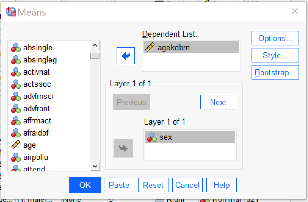
The most basic way to look at differences between groups is by using the Compare Means command, found by going to Analyze → Compare Means → Means (Alt+A, Alt+M, Alt+M). Put the independent (discrete) variable in the Layer 1 of 1 box and the dependent (continuous) variable in the Dependent List box. Note that while you can use as many independent and dependent variables as you would like in one Compare Means command, Compare Means does not permit for multivariate analysis, so including more variables will just mean more paired analyses (one independent and one dependent variable at a time) will be produced. Under Options, you can select additional statistics to produce; the default is the mean, standard deviation, and number of cases, but other descriptive and explanatory statistics are also available. The options under Style and Bootstrap are beyond the scope of this text. One the Compare Means test is set up, click ok.
The results that appear in the Output window are quite simple: just a table listing the statistics of the dependent variable that were selected (or, if no changes were made, the default statistics as discussed above) for each category or attribute of the independent variable. In this case, we looked at the independent variable SEX and the dependent variable AGEKDBRN to see if there is a difference between the age at which men’s and women’s first child was born.
| R’s age when their 1st child was born | |||
|---|---|---|---|
| Respondent’s sex | Mean | N | Std. Deviation |
| male | 27.27 | 1146 | 6.108 |
| female | 24.24 | 1601 | 5.917 |
| Total | 25.51 | 2747 | 6.179 |
Table 1, the result of this analysis, shows that the average male respondent had their first child at age 27.27, while the average female respondent had her first child at the age of 24.24, or about a three year difference. The higher standard deviation for men tells us that there is more variation in when men have their first child than there is among women.
The Compare Means command can be used with discrete independent variables with any number of categories, though keep in mind that if the number of respondents in each group becomes too small, means may reflect random variation rather than real differences.
Boxplots
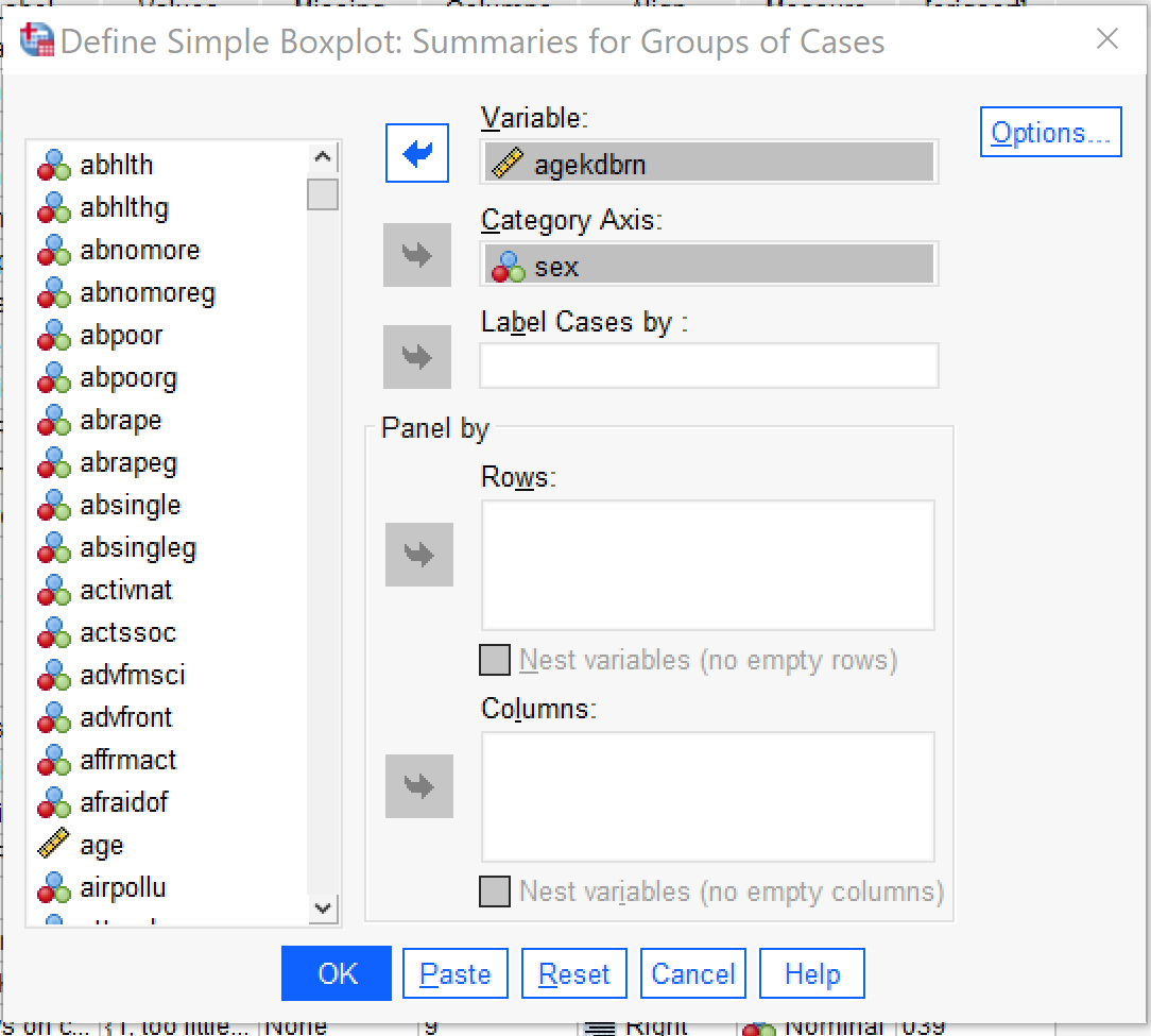
Boxplots provide a way to look at this same type of relationship visually. Like Compare Means, boxplots can be used with discrete independent variables with any number of categories, though the graphs will likely become illegible when the independent variable has more than 10 or so categories. To produce a boxplot, go to Graphs → Legacy Dialogs → Boxplot (Alt+G, Alt+L, Alt+X). Click Define. Then put the discrete independent variable in the Category Axis box and the continuous dependent variable in the Variable box. Under Options it is possible to include missing values to see if those respondents differ from those who did respond, but this option is not usually selected. Other options in the Boxplot dialog generally increase the complexity of the graph in ways that may make it harder to use, so just click OK once your variables are set up.
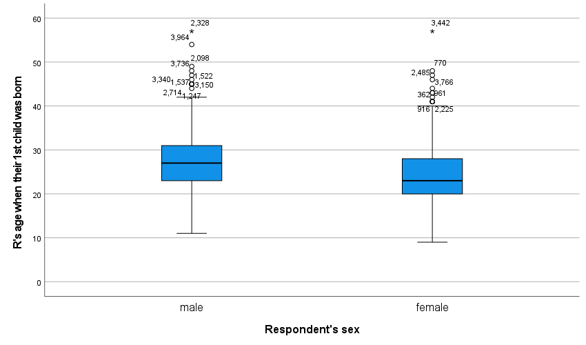
Figure 3 displays the boxplot that is produced. It shows that the median (the thick black line), the 25th percentile (the bottom of the blue box), the 75th percentile (the top of the blue box), the low end extreme (the ⊥at the bottom of the distribution) and the high end extreme before outliers (the T at the top of the distribution) are all higher for men than women, while the most extreme outlier (the *) is pretty similar for both. Outliers are labeled with their case numbers so they can be located within the dataset. As you can see, the boxplot provides a way to describe the differences between groups visually.
T-Tests For Statistical Significance
But what if we want to know if these differences are statistically significant? That is where T-tests come in. Like the Chi square test, the T test is designed to determine statistical significance, but here, what the test is examining is whether there is a statistically significant difference between the means of two groups. It can only be used to compare two groups, not more than two. There are multiple types of T tests; we will begin here with the independent-samples T test, which is used to compare the means of two groups of different people.
The computation behind the T test involves the standard deviation for each category, the number of observations (or respondents) in each category, and taking the mean value for each category and computing the difference between the means (the mean difference). Like in the case of the Chi square, this produces a calculated T value and degrees of freedom that are then compared to a table of critical values to produce a statistical significance value. While SPSS will display many of the figures computed as part of this process, it produces the significance value itself so there is no need to do any part of the computation by hand.
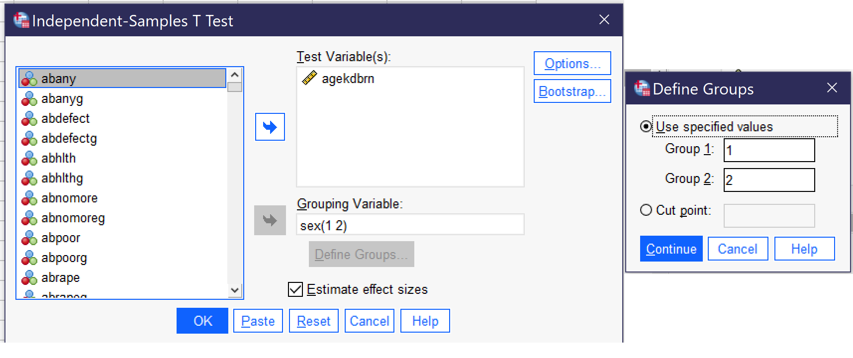
To produce an independent samples T test, go to go to Analyze → Compare Means → Independent-Samples T Test (Alt+A, Alt+M, Alt+T). Put the continuous dependent variable in the Test Variable(s) box. Note that you can use multiple continuous dependent variables at once, but you will only be looking at differences in each one, one at a time, not at the relationships between them. Then, put the discrete independent variable in the Grouping Variable box. Click the Define Groups button, and specify the numerical values of the two groups you wish to compare[1]—keep in mind that any one T test can only compare two values, not more, so if you have a discrete variable with more than two categories, you will need to perform multiple T tests or choose another method of analysis.[2] In most cases, other options should be left as they are. For our analysis looking at differences in the age a respondent’s first child was born in terms of whether the respondent is male or female, the Independent-Samples T Test dialogs would look as shown in Figure 4. AGEKDBRN is the test variable and SEX is the grouping variable, and under Define Groups, the values of 1 and 2 (the two values of the SEX variable) are entered. If we were using a variable with more than two groups, we would need to select the two groups we were interested in comparing and input the numerical values for just those two groups.
After clicking OK to run the test, the results are produced in the output window. While multiple tables are produced, the ones most important to the analysis are called Group Statistics and Independent Samples Test, and for our analysis of sex and age at the birth of the first child, they are reproduced below as Table 2 and Table 3, respectively.
| Respondent’s sex | N | Mean | Std. Deviation | Std. Error Mean | |
|---|---|---|---|---|---|
| R’s age when their 1st child was born | male | 1146 | 27.27 | 6.108 | .180 |
| female | 1601 | 24.24 | 5.917 | .148 |
Table 2 provides the number of respondents in each group (male and female), the mean age at the birth of the first child, the standard deviation, and the standard error of the mean, statistics much like those we produced in the Compare Means analysis above.
| Levene’s Test for Equality of Variances | t-test for Equality of Means | ||||||||||
|---|---|---|---|---|---|---|---|---|---|---|---|
| F | Sig. | t | df | Significance | Mean Difference | Std. Error Difference | 95% Confidence Interval of the Difference | ||||
| One-Sided p | Two-Sided p | Lower | Upper | ||||||||
| R’s age when their 1st child was born | Equal variances assumed | 1.409 | .235 | 13.026 | 2745 | <.001 | <.001 | 3.023 | .232 | 2.568 | 3.478 |
| Equal variances not assumed | 12.957 | 2418.993 | <.001 | <.001 | 3.023 | .233 | 2.565 | 3.480 | |||
Table 3 shows the results of the T test, including the T test result, degrees of freedom, and confidence intervals. There are two rows, one for when equal variances are assumed and one for when equal variances are not assumed. If the significance under “Sig.” is below 0.05, that means we should assume the variances are not equal and proceed with our analysis using the bottom row. If the significance under “Sig.” is 0.05 or above, we should treat the variances as equal and proceed using the top row. Thus, looking further at the top row, we can see the mean difference of 3.023 (which recalls the mean difference from our compare means analysis above) and the significance. Separate significance values are produced for one-sided and two-sided tests, though these are often similar. One-sided tests only look for change in one direction (increase or decrease), while two-sided tests look for any change or difference. Here, we can see both significance values are less than 0.001, so we can conclude that the observed mean difference of 3.023 does represent a statistically significant difference in the age at which men and women have their first child.
There are a number of other types of T tests. For example, the Paired Samples T Test is used when comparing two means from the same group—such as if we wanted to compare the average score on test one to the average score on test two given to the same students. There is also a One-Sample T Test, which permits analysts to compare observed data from a sample to a hypothesized value. For instance, a researcher might record the speed of drivers on a given road and compare that speed to the posted speed limit to see if drivers are going statistically significantly faster. To produce a Paired Samples T Test, go to Analyze → Compare Means → Paired-Samples T Test (Alt+A, Alt+M, Alt+P); the procedure and interpretation is beyond the scope of this text.
To produce a One-Sample T Test, go to Analyze → Compare Means → One-Sample T Test (Alt+A, Alt+M, Alt+S). Put the continuous variable of interest in the Test Variables box (Alt+T) and the comparison value in the Test Value box (Alt+V). In most cases, other options should be left as is. The results will show the sample mean, mean difference (the difference between the sample mean and the test value), and confidence intervals for the difference, as well as statistical significance tests both one-sided and two-sided. If the results are significant, that tells us that there is high likelihood that our sample differs from our predicted value; if the results are not significant, that tells us that any difference between our sample and our predicted value is likely to have occurred by chance, usually because the difference is quite small.
ANOVA
While a detailed discussion of ANOVA—Analysis of Variance—is beyond the scope of this text, it is another type of test that examines relationships between discrete independent variables and continuous dependent variables. Used more often in psychology than in sociology, ANOVA relies on the statistical F test rather than the T test discussed above. It enables analysts to use more than two categories of an independent variable—and to look at multiple independent variables together (including by using interaction effects to look at how two different independent variables together might impact the dependent variable). It also, as its name implies, includes an analysis of differences in variance between groups rather than only comparing means. To produce a simple ANOVA, with just one independent variable in SPSS, go to Analyze → Compare Means → One Way ANOVA (Alt+A, Alt+M, Alt+O); the independent variable in ANOVA is called the “Factor.” You can also use the Compare Means dialog discussed above to produce ANOVA statistics and eta as a measure of association by selecting the checkbox under Options. For more on ANOVA, consult a more advanced methods text or one in the field of psychology or behavioral science.
Exercises
- Select a discrete independent variable of interest and a continuous dependent variable of interest. Run appropriate descriptive statistics for them both and summarize what you have found.
- Run Compare Means and a Boxplot for your pair of variables and summarize what you have found.
- Select two categories of the independent variable that you wish to compare and determine what the numerical codes for those categories are.
- Run an independent-samples T test comparing those two categories and summarize what you have found. Be sure to discuss both statistical significance and the mean difference.
Media Attributions
- compare means © IBM SPSS is licensed under a All Rights Reserved license
- boxplot dialog © IBM SPSS is licensed under a All Rights Reserved license
- boxplot © IBM SPSS is licensed under a All Rights Reserved license
- independent samples t test dialog © IBM SPSS is licensed under a All Rights Reserved license
A variable measured using categories rather than numbers, including binary/dichotomous, nominal, and ordinal variables.
A statistical test designed to measure differences between groups.
