Quantitative Data Analysis With SPSS
12 Quantitative Analysis with SPSS: Data Management
Mikaila Mariel Lemonik Arthur
This chapter is designed to introduce a variety of ways to work with datasets and variables that facilitate analysis. None of the approaches in this chapter themselves produce results, but rather are designed to enable analysis that might not be possible if datasets are used in their default form. First, it will show how to perform analysis on more limited subsets of data. Then, it will show how to transform variables to change their level of measurement, reduce attributes, create index variables, and otherwise combine variables. One quick note about a topic that is not covered in this text: the application of survey weights. More advanced quantitative analysts will want to learn to properly weight their data before performing analysis.
Working With Datasets
In some cases, analysts may wish to use a smaller subset of their dataset or to analyze different groups within the dataset separately. This section of the chapter will review select cases and split file, approaches for doing just this.
Select Cases

The Select Cases tool permits analysts to choose a subset of cases upon which to perform analysis. It can be found at the bottom of the Data menu (Alt+D, Alt+S); the Select Cases dialog is shown in Figure 1. Select cases offers the option of selecting cases based on satisfying a certain condition (e.g. cases with a specific value for a specific variable), selecting a random sample of a percentage or number of cases, selecting a specific range of cases, or using a filter variable to select only those cases with a value other than 0 or missing on that variable.
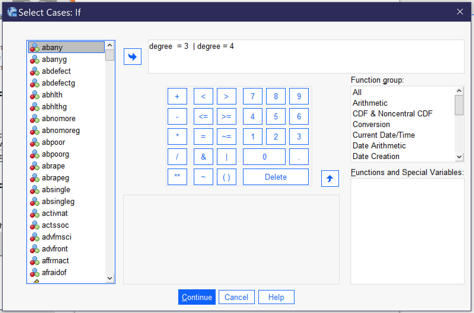
When using the “If condition is satisfied” option, click the “If…” button and use variable names and logical or mathematical operators to write an expression (either by clicking or just typing the expression). For instance, one might select only those who have a bachelor’s degree or higher by writing [latex]degree = 3 \ | \ degree = 4[/latex],[1] as shown in Figure 2.
Once an option has been selected, analysts then need to determine what should happen to the selected cases. They can choose to filter out the unselected cases or to copy the selected cases into a new file with a given filename. SPSS also permits the option of deleting unselected cases, but since this permanently alters the original dataset, it is not recommended. If “Filter Out Unselected Cases” is chosen, it is important to remember to return to the Select Cases dialog when the portion of the project relying on the selected subset of cases is completed. When returning to Select Cases, “All Cases” should be selected in order to revert to the original dataset with all cases available for analysis.
Split File
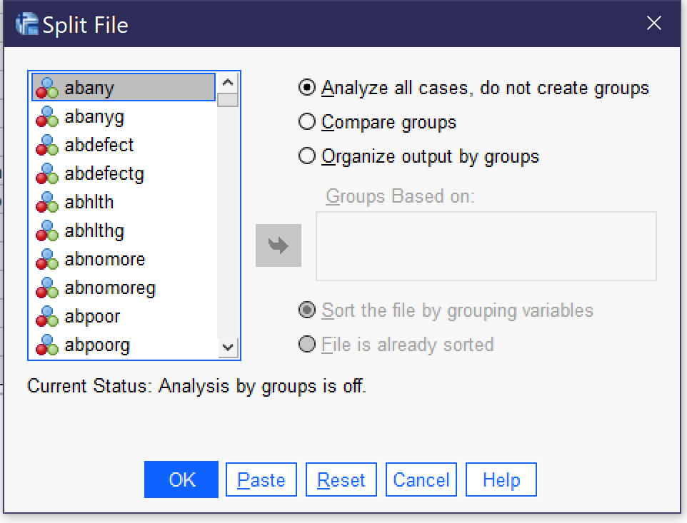
The split file tool allows analysts to produce output that is separated according to the attributes of a variable. For instance, analysts could perform descriptive statistics or crosstabulations and generate separate output for different race, sex, educational, or other categories. Split file can be accessed via the Data menu (Alt+D, Alt+F); the dialog is shown in Figure 3. Analysts can choose to analyze all cases (not splitting the file) or to split the file and either compare groups or organize output by groups. Using each of these options, all analyses performed appear in the output in multiple copies, one for each of the attributes of the selected variable. So, for instance, if the file were split by SEX (in the 2021 GSS, SEX only has the attributes of male and female), separate descriptive statistics, crosstabs, graphs, or whatever other output is desired will be produced. The difference between “Compare groups” and “Organize output by groups” is that “Compare groups” produces a stack of output—say, the frequencies tables for male and female—right on top of each other, while “Organize output by groups” produces all output requested in a single procedure separated for each attribute.
Once the analyst has selected one of these options, they select the variable and use the blue arrow to put it in the Groups Based on box; in most cases, the option for Sort the file by grouping variables should be selected as well. Then click on and proceed to perform the desired analysis. Once the analysis is completed, return to the Compare Groups dialog and select “Analyze all cases, do not compare groups” and click OK so that the split file is turned off.
Working With Variables
Analysts may wish to use variables differently than the way they were originally collected. This section of the chapter will address three approaches for transforming variables: first, recoding variables, which permits transforming a continuous variable into an ordinal one or reducing the number of attributes in a variable to fewer, larger categories; second, creating indexes by combining variables using the count function; and third, using compute to manipulate or combine variables in other ways, such as creating averages.
Recoding
Recoding is a procedure that permits analysts to change the way in which the attributes of a variable are set up. It can be used for a variety of purposes, among them:
- Converting a continuous variable into an ordinal one by grouping numerical values into categories,
- Simplifying a nominal or ordinal variable with many categories by collapsing those categories into a smaller number of categories,
- Changing the direction of a variable, for instance taking an ordinal variable with 5 categories ranging from 1: strongly disagree to 5: strongly agree and turning it into an ordinal variable with 5 categories ranging from 1: strongly agree to 5: strongly disagree, and
- Creating dummy variables, as will be discussed in the chapter on multivariate regression.
This section of the chapter will provide examples of how to conduct the first two types of recoding. Note that before proceeding to recode any variable, it is essential to first produce complete descriptive statistics for the variable in question and study them carefully. If you are recoding a continuous variable, you may wish to use the “cut points” option under Analyze → Descriptive Statistics → Frequencies → Statistics, being sure to specify the number of equal groups you are considering creating. If you are recoding a discrete variable it is also essential to understand what the attributes (value labels) are for that variable and how they are coded (values). Take good notes on both the descriptive statistics and the attributes so that you have the information available to help you decide how to set up your recode.
The recode dialog is found under Transform (Alt+T). Note that there are several different recoding options. You should never use Recode into Same Variables (Alt+S), as this writes over your original data. The Automatic Recode (Alt+A) option is most useful when data is in non-numeric form and needs to be converted to numeric form. Most frequently, as a quantitative analyst, you will use Recode into Different Variables (Alt+R).
Recoding a Continuous Variable into an Ordinal Variable
| Age of respondent | ||
|---|---|---|
| N | Valid | 3699 |
| Missing | 333 | |
| Mean | 52.16 | |
| Median | 53.00 | |
| Std. Deviation | 17.233 | |
| Variance | 296.988 | |
| Skewness | .018 | |
| Std. Error of Skewness | .040 | |
| Kurtosis | -1.018 | |
| Std. Error of Kurtosis | .080 | |
| Range | 71 | |
| Minimum | 18 | |
| Maximum | 89 | |
| Percentiles | 20 | 35.00 |
| 40 | 46.00 | |
| 60 | 59.00 | |
| 80 | 69.00 | |
Let’s say we would like to recode AGE, changing it from a continous variable to a discrete variable. We might use our own understanding of ages to come up with categories, like 18-25, 26-35, 36-45, 46-55, 56-65, 66-75, and 75 and older. But these categories, it turns out, might not be so useful, as not very many people in our dataset are at the youngest or oldest ends of the distribution—something we find out if we look at the descriptive statistics. In fact, if we produce descriptive statistics using cut points for five equal groups—as shown in Table 1, we would find out that we have to get all the way to age 35 to have 20% of the people in our sample fall into one age category. We might not want to just use the cut points our descriptive statistics found, though, as they do not necessarily make sense as theoretical groupings. Perhaps instead we would choose 18-35, 36-45, 46-59, 60-69, and 70 and older. These grouping would be approximately equal in size, but make more sense numerically. Once we determine our groups, we also need to decide which numerical value we will assign each group—perhaps 1:18-35, 2:36-45; 3:46-59, 4:60-69; 5:70+. Now that we have decided how we will recode our variable, we are ready to proceed with actually recoding the variable.
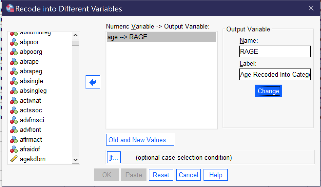
To begin the process of recoding, go to Transform → Recode Into Different. Select the variable you wish to recode and move it into the box using the blue arrow. Then, give the variable a new name and label. Many analysts use the convention of adding an R to the original variable name, thus here we are giving our variable the new name RAGE and the label “Age Recoded Into Categories.” Click the Change button. There is an If… option for more complicated recoding procedures, but in most cases all that needs to be done now is clicking Old and New Values to put in the old and new values we already decided upon.
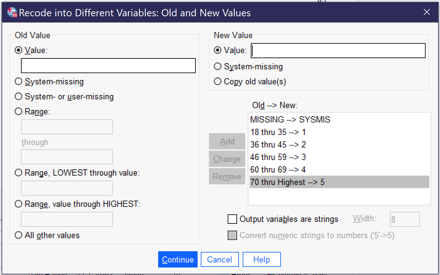
In the Old and New Values dialog, there are a variety of ways to indicate the original value (old) and the new value. We always begin by selecting old value: System or user-missing and new value: System-missing, to ensure that missing values remain missing. We then put in the rest of our categories using the Range ____ through _____ option, except for the final category, where we use Range, value through highest to ensure we don’t accidentally leave out those 89-year-olds. Once an old value and its respective new value have been entered, we click the Add button so that they appear in the Old → New box. In other cases, analysts might change individual values, use Range, lowest through value, or combine all other values. If it is necessary to edit or delete something that has already been added, use the Change (to edit) or Remove (to delete) buttons. When all of the old and new values have been added, the Old and New Values dialog should look as it does in Figure 5, with the following test in the Old → New box:
MISSING-->SYSMIS 18 thru 35-->1 36 thru 45-->2 46 thru 59-->3 60 thru 69-->4 70 thru highest-->5 |
When everything is set up, click Continue and then OK. To see your new variable, scroll to the bottom of the screen in Variable View.
There is one more step to recoding, and that is to add the value labels. To do this, go to Variable View; you will most likely find your new variable at the very bottom of the list of variables. If you click in the Values box for the row with your new variable in it, as shown in Figure 6, you will see a box with … in it. Click the … and the value labels dialog will come up.

To enter the value labels, click on the green plus sign, and then enter a numerical value and its associated value label. Click the plus sign again to enter the next value and value label, and so on until all have been entered. If you need to remove one that has been entered incorrectly, use the red X. There is a spellchecker if useful. When you are done, the Value Labels dialog should look as it does in Figure 7. Then click OK, and remember to save your dataset so that you don’t lose your new variable.

Finally, it is time to check that the recoding is proceeding correctly before using the new variable in any analysis. To check the variable, produce a frequency distribution. Assess the frequency distribution for evidence of any errors, such as:
- Old values that did not get caught in the recoding process,
- Categories that are missing from the new values,
- More missing values than would be expected, and
- Unexpected discrepancies between the descriptive statistics from the original variable and those produced now.
| Frequency | Percent | Valid Percent | Cumulative Percent | ||
|---|---|---|---|---|---|
| Valid | 18-35 | 795 | 19.7 | 21.5 | 21.5 |
| 36-45 | 643 | 15.9 | 17.4 | 38.9 | |
| 46-59 | 855 | 21.2 | 23.1 | 62.0 | |
| 60-69 | 728 | 18.1 | 19.7 | 81.7 | |
| 70+ | 678 | 16.8 | 18.3 | 100.0 | |
| Total | 3699 | 91.7 | 100.0 | ||
| Missing | System | 333 | 8.3 | ||
| Total | 4032 | 100.0 | |||
In the case of our RAGE variable, we can observe in Table 2 that we did a relatively good job of keeping the proportion of respondents in each of our categories pretty even. In the absence of theoretical or conceptual reasons for choosing a particular recoding strategy, making categories of relatively consistent size can be a good way to proceed.
Reducing the Attributes of a Discrete Variable
As noted above, recoding can also be used to condense categories in the case of an ordinal or nominal variable with many categories. The example here uses the variable POLVIEWS, an ordinal variable measuring respondents’ political views on a seven-point scale from extremely liberal to extremely conservative. In recoding this variable, we might want to reduce the seven points to three: liberal, moderate, and conservative. But which values belong in which categories? We might say that extremely liberal and liberal make up the liberal category; extremely conservative and conservative make up the conservative category; and slightly liberal, slightly conservative, and moderate/middle of the road make up the moderate category. So we produce a frequency table to see what our data looks like. This frequency table is shown in Table 3.
| Frequency | Percent | Valid Percent | Cumulative Percent | ||
|---|---|---|---|---|---|
| Valid | extremely liberal | 207 | 5.1 | 5.2 | 5.2 |
| liberal | 623 | 15.5 | 15.7 | 20.9 | |
| slightly liberal | 490 | 12.2 | 12.4 | 33.3 | |
| moderate, middle of the road | 1377 | 34.2 | 34.7 | 68.0 | |
| slightly conservative | 476 | 11.8 | 12.0 | 80.0 | |
| conservative | 617 | 15.3 | 15.6 | 95.6 | |
| extremely conservative | 174 | 4.3 | 4.4 | 100.0 | |
| Total | 3964 | 98.3 | 100.0 | ||
| Missing | System | 68 | 1.7 | ||
| Total | 4032 | 100.0 | |||
Table 3 might cause us to think that our original idea about how to combine these categories is not the best, given how few people would end up in the liberal and conservative categories and how many in the moderate category. Instead, we might conclude that it would make more sense to group extremely liberal, liberal, and slightly liberal together; keep moderate on its own; and then group extremely conservative, conservative, and slightly conservative together. And we might decide that 1 will be liberal, 2 will be moderate, and 3 will be conservative. We also need to write down the value labels from our existing variable so that we can use them in the recoding.
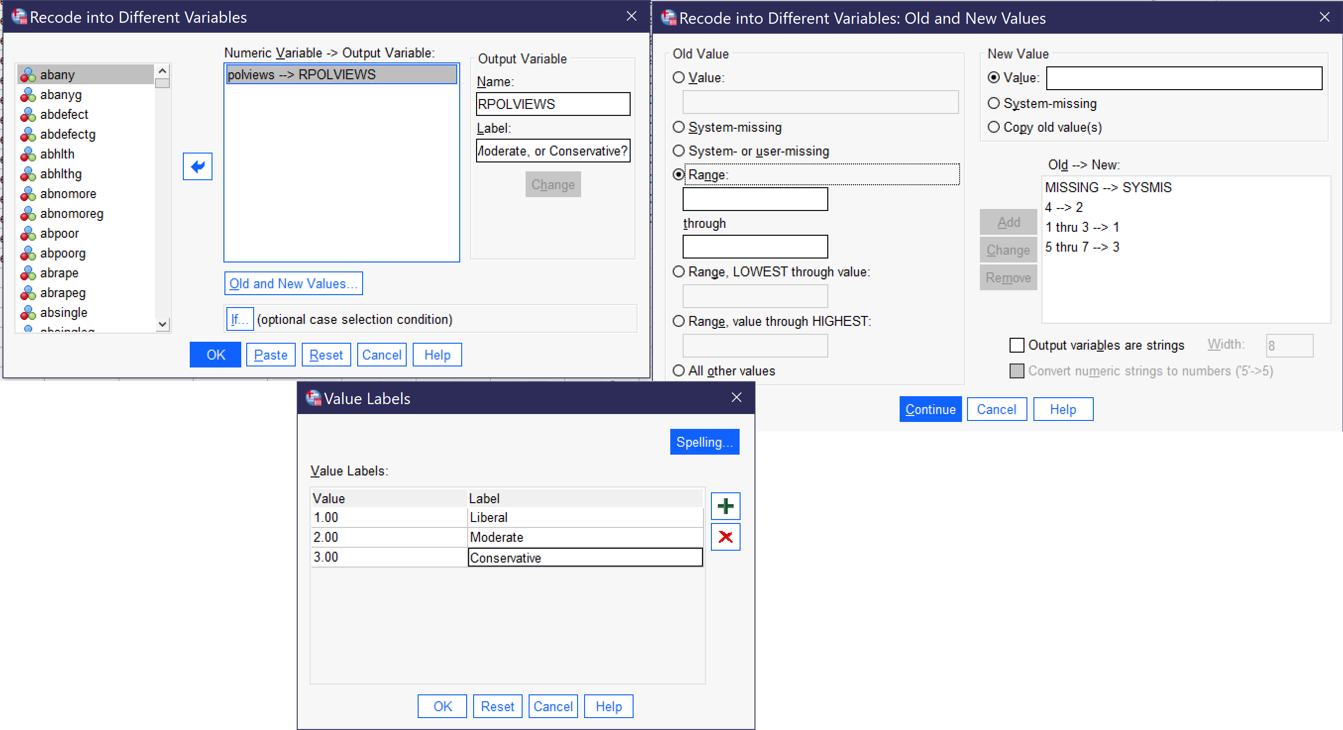
Once we’ve made these decisions, it’s time to proceed with the recoding, which we do much the same way as we did for the recoding of the continuous variable above, by going to Transform → Recode Into Different. Give the variable a new name, RPOLVIEWS, and a new label, Is R Liberal, Moderate, or Conservative? Click Change, and then click Old and New Values. Note that if you are recoding right after recoding a prior variable, you will need to use the Remove button to remove the old and new values from the prior recoding process. The old and new values we will be entering are shown below; Figure 8 shows what the recode dialogs should look like.
MISSING-->SYSMIS 1 thru 3-->1 4-->2 5 thru 7-->3 |
Once the old and new values are entered, click Continue and then OK. Then, scroll to the new variable in Variable View and add the value labels: 1 Liberal, 2 Moderate, 3 Conservative, as shown in Figure 8.
Finally, produce a frequency table to check for errors before using the new RPOLVIEWS variable in an analysis. As Table 4 shows, the recoding strategy we chose happened to distribute respondents quite evenly, though of course it is based on conceptual concerns rather than simply the distribution of respondents.
| Frequency | Percent | Valid Percent | Cumulative Percent | ||
|---|---|---|---|---|---|
| Valid | Liberal | 1320 | 32.7 | 33.3 | 33.3 |
| Moderate | 1377 | 34.2 | 34.7 | 68.0 | |
| Conservative | 1267 | 31.4 | 32.0 | 100.0 | |
| Total | 3964 | 98.3 | 100.0 | ||
| Missing | System | 68 | 1.7 | ||
| Total | 4032 | 100.0 | |||
Creating an Index
In the course of many research and data analysis projects, researchers may seek to create index variables by combining responses on multiple related variables. While it may seem that simply adding the values together might work, one of the main reasons simply adding does not work is that it cannot distinguish between circumstances where a respondent did not answer one or more questions and circumstances in which respondents gave answers with lower numerical values. Therefore, the process to be detailed here requires two steps: first, collecting missing responses, and then, creating an index while excluding those respondents who did not answer all questions included in the index.
The example index detailed here is an index of the seven variables in the 2021 GSS that ask respondents their views on whether abortion should be legal in a variety of circumstances: in the case of fetal defect (ABDEFECT), risks to health (ABHLTH), rape (ABRAPE), if the pregnant person is single (ABSINGLE), if the pregnant person is poor (ABPOOR), if the pregnant person already has children and does not want any more (ABNOMORE), and for any reason (ABANY). Note that in the 2021 GSS there are a separate set of variables asking about abortion that end in G. These variables reflect differences in wording as part of a survey experiment; one could use them instead of the non-G abortion opinion variables, but the two sets should not be combined as they were asked of different people.
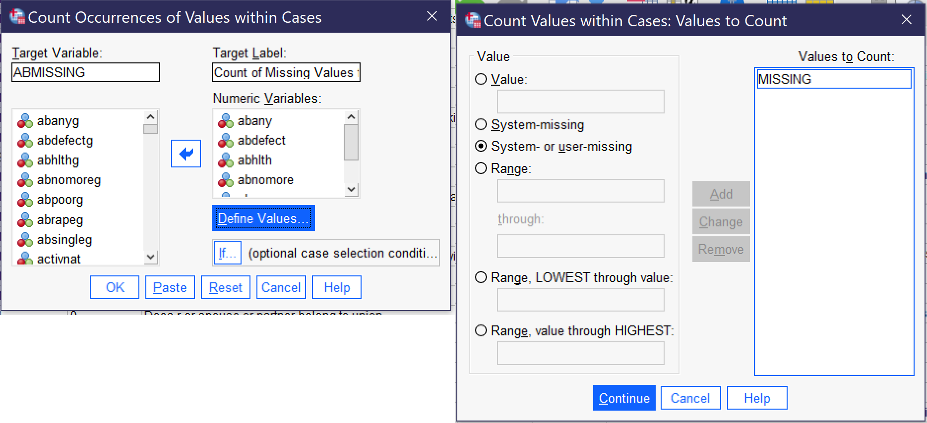
Our first task is to look at the value labels for our variables. Each of these abortion variables is coded with 1:Yes and 2:No; we need to determine whether we wish to make an index of yeses or nos, and in this case we will use the Yeses. The second task is to collect the missing responses so that we can exclude them. Both this part of the process and the ultimate task of creating the index utilize Transform → Count Values Within Cases… (Alt+T, Alt+O). Once the Count dialog is open, we need to give our new variable a name (in the Target Variable box) and Label (in the Target Label box). We will call this variable ABMISSING with the label Count of Missing Variables for Abortion Variables, given that’s what we are counting at the moment. We then move all of the variables (seven, in this case) we are including in our index into the Variables box using the blue arrow. Next, click on the Define Values button. Select the radio button next to System- or user-missing and click Add, then click Continue, then click OK. Figure 9 shows how this Count procedure should be set up.
| Frequency | Percent | Valid Percent | Cumulative Percent | ||
|---|---|---|---|---|---|
| Valid | .00 | 1284 | 31.8 | 31.8 | 31.8 |
| 1.00 | 118 | 2.9 | 2.9 | 34.8 | |
| 2.00 | 26 | .6 | .6 | 35.4 | |
| 3.00 | 8 | .2 | .2 | 35.6 | |
| 4.00 | 9 | .2 | .2 | 35.8 | |
| 5.00 | 1 | .0 | .0 | 35.9 | |
| 6.00 | 11 | .3 | .3 | 36.1 | |
| 7.00 | 2575 | 63.9 | 63.9 | 100.0 | |
| Total | 4032 | 100.0 | 100.0 | ||
It is a good practice to produce a frequency table at this stage to check for errors and ensure that a reasonable number of cases remain for use in producing the desired index variable. In this example, the frequency table for the missing values count should appear as in Table 5. This shows that 31.8%, or 1284 cases, answered all seven abortion questions and thus will be able to be included in our index variable. 63.9% did not answer any of the seven questions (presumably because they were not asked them), while a far smaller percent answered only some of the questions—and thus also will be excluded from our index.
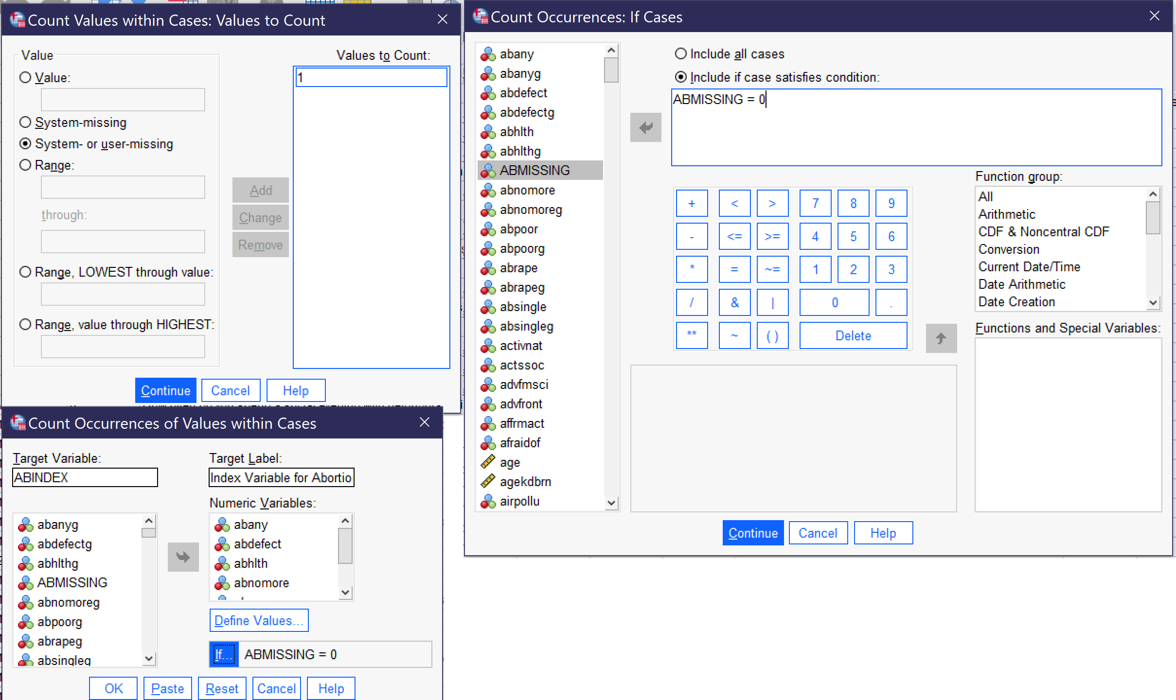
The next step is to create the index variable while excluding those who have missing values. To do this, we again go to Transform → Count Values Within Cases…. This time, we will call our new variable ABINDEX and give it the label Index Variable for Abortion Questions. Under Define Values, we remove MISSING and, in its place, add 1 to the Values to Count box, and then click Continue. Next, we click If… and select the radio button next to Include if case satisfies condition. In the box, we say ABINDEX = 0 (so that cases in which any of the included variables have missing values are excluded) and click Continue. Figure 10 below shows what all of the dialogs should look like when everything is set up to produce the index. Once everything is ready, click OK.
Finally, produce a frequency distribution for the new index variable. (Note: some analysts treat this type of index variable as ordinal, while others argue that because it is a count of numbers it might better be understood as continuous. Either approach is acceptable for producing descriptive statistics.) Table 6 shows the results, which many people might find surprising: 50.4% of respondents—just a tad more than half—agree that abortion should be legal in all of the cases about which they were asked, while only 7.2% believe abortion should be legal in none of them.
| Frequency | Percent | Valid Percent | Cumulative Percent | ||
|---|---|---|---|---|---|
| Valid | .00 | 93 | 2.3 | 7.2 | 7.2 |
| 1.00 | 82 | 2.0 | 6.4 | 13.6 | |
| 2.00 | 104 | 2.6 | 8.1 | 21.7 | |
| 3.00 | 172 | 4.3 | 13.4 | 35.1 | |
| 4.00 | 69 | 1.7 | 5.4 | 40.5 | |
| 5.00 | 43 | 1.1 | 3.3 | 43.8 | |
| 6.00 | 74 | 1.8 | 5.8 | 49.6 | |
| 7.00 | 647 | 16.0 | 50.4 | 100.0 | |
| Total | 1284 | 31.8 | 100.0 | ||
| Missing | System | 2748 | 68.2 | ||
| Total | 4032 | 100.0 | |||
Computing Variables
Sometimes, analysts want to combine variables in ways other than by making an index (for instance, adding two continuous variables together or taking their average) or otherwise wish to perform mathematical functions on them. These types of operations can be conducted by going to Transform → Compute Variable (Alt+T, Alt+C). Here, we will try two examples, one in which we take the average of the two variables measuring parental occupational prestige (MAPRES10 and PAPRES10) to determine respondents’ parents’ average occupational prestige, and one in which we take a continuous variable collected on a weekly basis (WWWHR, which measures how many hours respondents spend on the Internet per day) and divide it by seven, the number of days in a week, to produce a variable on a daily basis (the average number of hours respondents spend on the internet per day).
To create the computed variable for average parental occupational prestige, we go to Transform → Compute Variable. We then indicate the name for our new variable in the Target Variable box; we will call it PARPRES10 (for parental prestige). Once we enter this, we can click on the Type & Label box to provide our variable with a label and be sure it is classified as a numeric variable. Next, under the Numeric Expression box, we set up the formula that will produce the outcome we want. Here, we are averaging two variables, so we want to add them together (remember the parentheses, for order of operations) and then divide by two, like this: [latex](mapres10\ +\ papres10)\ /\ 2[/latex]. The If… (optional case selection) can be used to only include or to make sure to exclude certain kinds of cases; we do not need to use it to exclude missing values, as the Compute function already excludes them from computation.
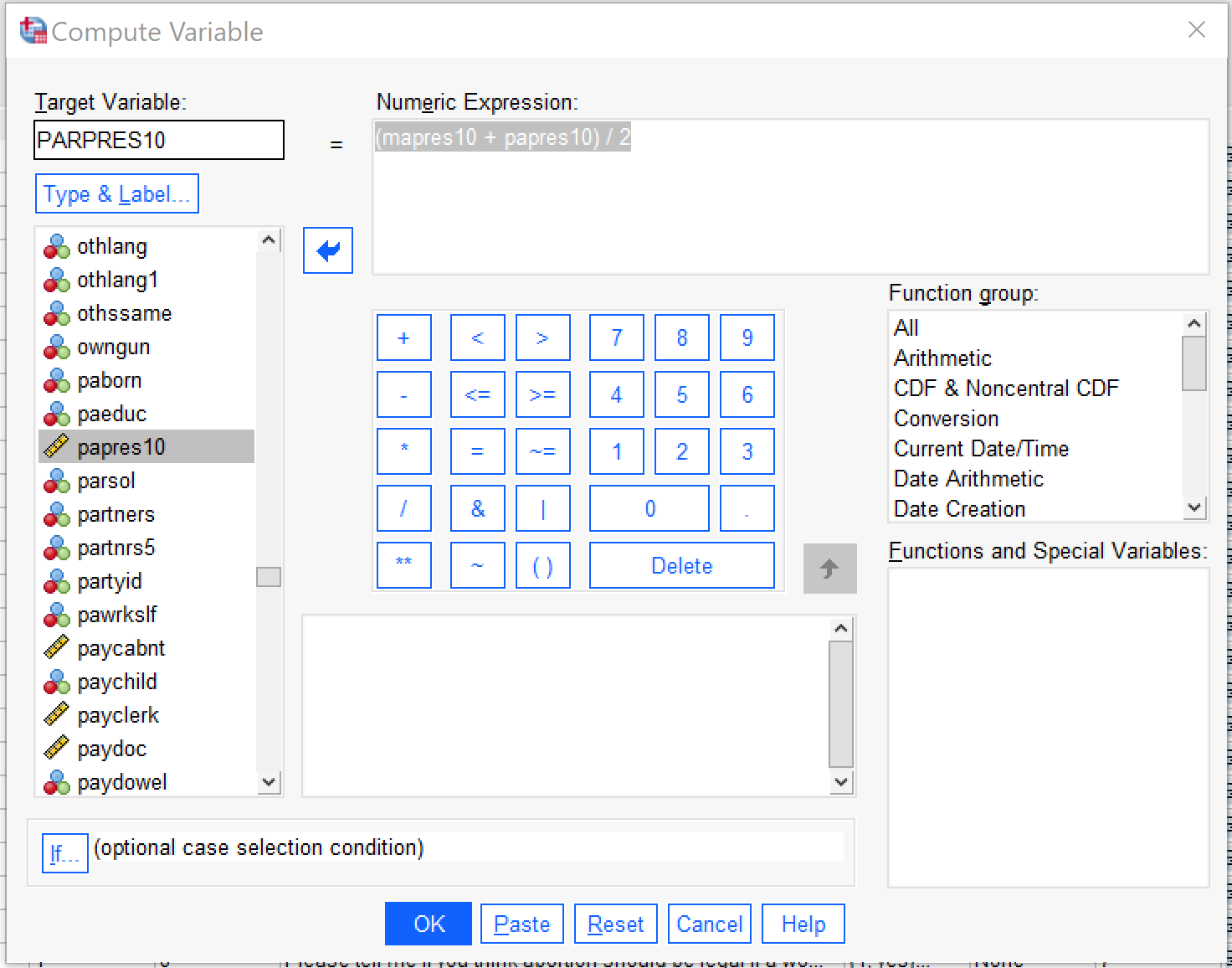
Figure 11 shows what the Compute Variable dialog should look like to produce the desired variable, the average of mother’s and father’s occupational prestige. When it is set up, click OK. The resulting variable is continuous, so the last step is to produce descriptive statistics for the continuous variable. Here, we will produce descriptive statistics for all three variables–the two original occupational prestige scores and our new average. Table 7 shows the results.
| Average of Mother’s and Father’s Occupational Prestige | Mothers occupational prestige score (2010) | Father’s occupational prestige score (2010) | ||
|---|---|---|---|---|
| N | Valid | 2232 | 2767 | 3349 |
| Missing | 1800 | 1265 | 683 | |
| Mean | 44.1633 | 42.66 | 45.16 | |
| Median | 42.5000 | 42.00 | 44.00 | |
| Std. Deviation | 10.58686 | 13.168 | 13.148 | |
| Variance | 112.082 | 173.387 | 172.869 | |
| Skewness | .493 | .389 | .622 | |
| Std. Error of Skewness | .052 | .047 | .042 | |
| Kurtosis | -.317 | -.672 | -.305 | |
| Std. Error of Kurtosis | .104 | .093 | .085 | |
| Range | 60.00 | 64 | 64 | |
| Minimum | 20.00 | 16 | 16 | |
| Maximum | 80.00 | 80 | 80 | |
| Percentiles | 25 | 36.0000 | 32.00 | 35.00 |
| 50 | 42.5000 | 42.00 | 44.00 | |
| 75 | 51.5000 | 50.00 | 52.00 | |
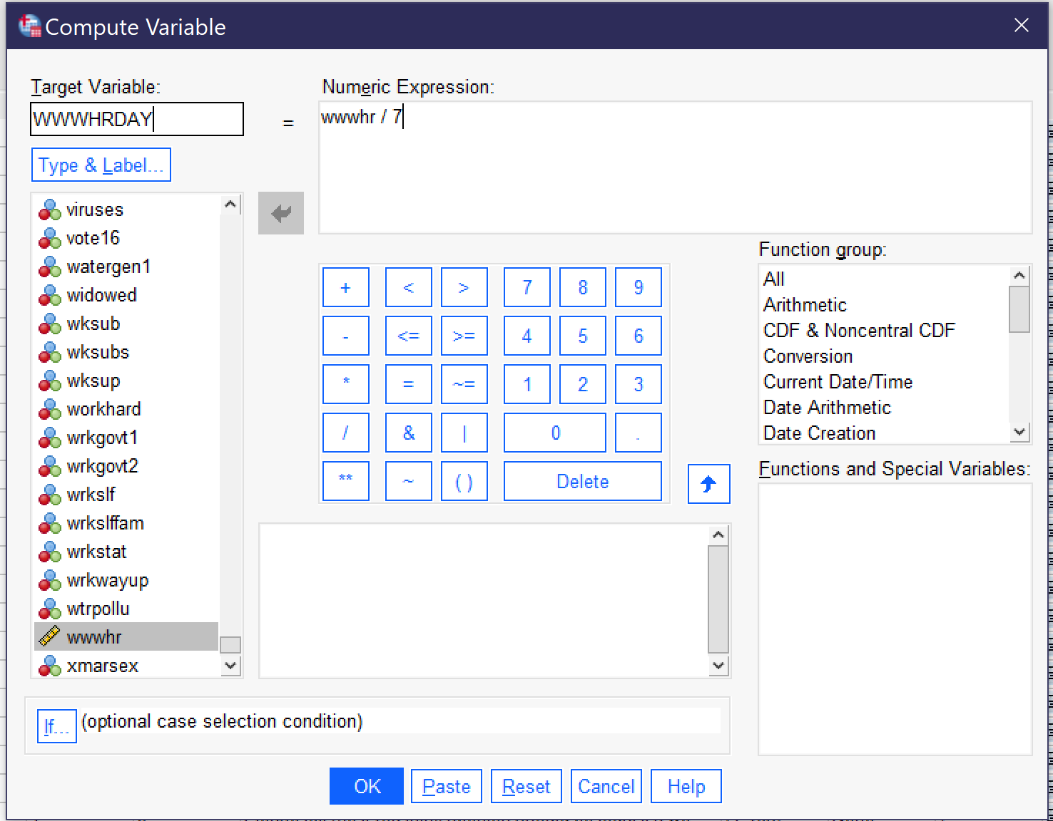
Let’s take one last example: starting with a variable that measures the number of hours respondents spend on the Internet per week and adjusting it so it measures the number of hours they spend per day. We will call the new variable WWWHRDAY, and the expression to produce it is simply [latex]wwwhr \ / \ 7[/latex], as shown in Figure 13. Then click OK.
Again, the final step is to compute descriptive statistics for the new variable, as shown in Table 8. These descriptive statistics show that the average person spends nearly 15 hours a week online, or just over 2 hours per day—but that this is pretty skewed by folks who spend quite a bit of time online, as the median time online is just 9 hours a week or somewhat over 1 hour per day. The range shows that there are people in the dataset who spend no time online at all, and others who claim to spend every hour of the day online (how is this possible? Don’t they sleep?). Looking at the percentiles, we can observe that a quarter of our respondents spend less than half an hour a day online, while another quarter claim to spend more than 2.8 hours per day online.
| Hours per week r spends on the Internet | Average Number of Hours Online Per Day | ||
|---|---|---|---|
| N | Valid | 2466 | 2466 |
| Missing | 1566 | 1566 | |
| Mean | 14.80 | 2.1146 | |
| Median | 9.00 | 1.2857 | |
| Std. Deviation | 17.392 | 2.48459 | |
| Variance | 302.487 | 6.173 | |
| Skewness | 2.575 | 2.575 | |
| Std. Error of Skewness | .049 | .049 | |
| Kurtosis | 10.257 | 10.257 | |
| Std. Error of Kurtosis | .099 | .099 | |
| Range | 168 | 24.00 | |
| Minimum | 0 | .00 | |
| Maximum | 168 | 24.00 | |
| Percentiles | 25 | 3.00 | .4286 |
| 50 | 9.00 | 1.2857 | |
| 75 | 20.00 | 2.8571 | |
Exercises
- Select cases to select only those who identify as poor (from the variable CLASS). Produce a histogram of working hours (from the variable HRS1). Then select all cases and produce the same histogram. Compare your results.
- Split file by RACE or SEX. Choose any variable of interest and perform appropriate descriptive statistics. Write a paragraph explaining the differences you observe between the racial or sex categories in your analysis.
- Recode HRS1, creating no more than 5 categories. Be sure you can explain why your categories are grouped the way they are, and look at the descriptive statistics as you determine them. Then produce descriptive statistics after recoding and summarize your results.
- Recode ENPRBUS, creating no more than 4 categories. Be sure you can explain why your categories are grouped the way they are, and look at the descriptive statistics as you determine them. Then produce descriptive statistics after recoding and summarize your results.
- Create an index of the six variables asking about whether people with various views should be allowed to speak in your community (SPKATH, SPKRAC, SPKCOM, SPKMIL, SPKHOMO, SPKMSLM), being sure to create the missing value index first. Produce appropriate descriptive statistics and summarize your results.
- Create a new variable for the average number of hours per day the respondent spends in a car or other vehicle by using the Compute function to divide CARHR (the number of hours in a vehicle per week) by 7. Produce descriptive statistics for the original CARHR variable and your new computed variable.
Media Attributions
- select cases © IBM SPSS is licensed under a All Rights Reserved license
- select cases if © IBM SPSS is licensed under a All Rights Reserved license
- split file © IBM SPSS is licensed under a All Rights Reserved license
- recode age © IBM SPSS is licensed under a All Rights Reserved license
- recode age values © IBM SPSS is licensed under a All Rights Reserved license
- to enter value labels © IBM SPSS is licensed under a All Rights Reserved license
- age value labels © IBM SPSS is licensed under a All Rights Reserved license
- recoding polviews © IBM SPSS is licensed under a All Rights Reserved license
- count of missing values © IBM SPSS is licensed under a All Rights Reserved license
- creating an index © IBM SPSS is licensed under a All Rights Reserved license
- compute average © IBM SPSS is licensed under a All Rights Reserved license
- compute math © IBM SPSS is licensed under a All Rights Reserved license
- Note: the symbol | means or in mathematical notation. ↵
A two-category (binary/dichotomous) variable that can be used in regression or correlation, typically with the values 0 and 1.
A composite variable created by combining information from multiple variables.
